Bonferroni correction calculator
Running several tests at once inflates the chance of a false positive. Enter α and the number of tests for the Bonferroni threshold, or paste your p-values to see Bonferroni, Holm and Benjamini–Hochberg adjustments side by side, with the tests each method rejects.
Separate with commas, spaces or new lines. Leave blank to get only the adjusted threshold.
┄ α = 0.05 (no correction) ┄ Benjamini–Hochberg iα/m ━ Holm α/(m − i + 1) ━ Bonferroni α/m = 0.00625 ━ p-values, smallest first
A p-value under a line is significant by that method (Holm and Benjamini–Hochberg are applied in order along the ranks). 1 p-value is above 0.1 and is drawn on the top edge.
| # | p | Rank | Bonferroni p | Bonf. | Holm p | Holm | BH p | BH |
|---|---|---|---|---|---|---|---|---|
| 1 | 0.001 | 1 | 0.008 | Reject | 0.008 | Reject | 0.008 | Reject |
| 2 | 0.008 | 2 | 0.064 | – | 0.056 | – | 0.032 | Reject |
| 3 | 0.039 | 3 | 0.312 | – | 0.234 | – | 0.0672 | – |
| 4 | 0.041 | 4 | 0.328 | – | 0.234 | – | 0.0672 | – |
| 5 | 0.042 | 5 | 0.336 | – | 0.234 | – | 0.0672 | – |
| 6 | 0.06 | 6 | 0.48 | – | 0.234 | – | 0.08 | – |
| 7 | 0.074 | 7 | 0.592 | – | 0.234 | – | 0.08457 | – |
| 8 | 0.205 | 8 | 1 | – | 0.234 | – | 0.205 | – |
Show the working, step by step
Bonferroni: multiply each p-value by m (cap at 1), or equivalently compare each p to α/m.
α/m = 0.05 ÷ 8 = 0.00625 smallest: 0.001 × 8 = 0.008
Holm: sort the p-values; multiply the i-th smallest by (m − i + 1), then carry the running maximum down the list so adjusted values never decrease.
p(1) = 0.001 × 8 = 0.008 p(2) = 0.008 × 7 = 0.056 p(3) = 0.039 × 6 = 0.234
Benjamini–Hochberg: multiply the i-th smallest by m/i, then carry the running minimum up from the largest.
p(1) = 0.001 × 8/1 = 0.008 p(2) = 0.008 × 8/2 = 0.032 p(3) = 0.039 × 8/3 = 0.104
Reject every hypothesis whose adjusted p is at or below α = 0.05.
Bonferroni and Holm control the family-wise error rate (the chance of any false positive). Holm always rejects at least as many as Bonferroni. Benjamini–Hochberg controls the false discovery rate instead, the expected share of false positives among the rejections, so it rejects more.
The formulas
Bonferroni: p_adj = min(1, m × p), or reject when p ≤ α/m Holm: p_adj(i) = max over j ≤ i of min(1, (m − j + 1) × p(j)) Benjamini–Hochberg: p_adj(i) = min over j ≥ i of min(1, m × p(j) / j)
Here p(1) ≤ p(2) ≤ … ≤ p(m) are the p-values sorted from smallest to largest. The running maximum in Holm and the running minimum in Benjamini–Hochberg keep the adjusted values in the same order as the raw ones. These are the same definitions R uses in p.adjust().
Why a correction is needed
If each of 8 independent tests has a 5% false-positive rate and every null hypothesis is true, the chance that at least one comes out significant is 1 − 0.95⁸ = 33.7%. Report the one that did and a third of the time you are reporting noise. A correction brings the family-wise rate back to 5%.
Worked example
A study compares a treatment with control on 8 outcomes and gets p-values 0.001, 0.008, 0.039, 0.041, 0.042, 0.060, 0.074 and 0.205. Without correction, five are below 0.05.
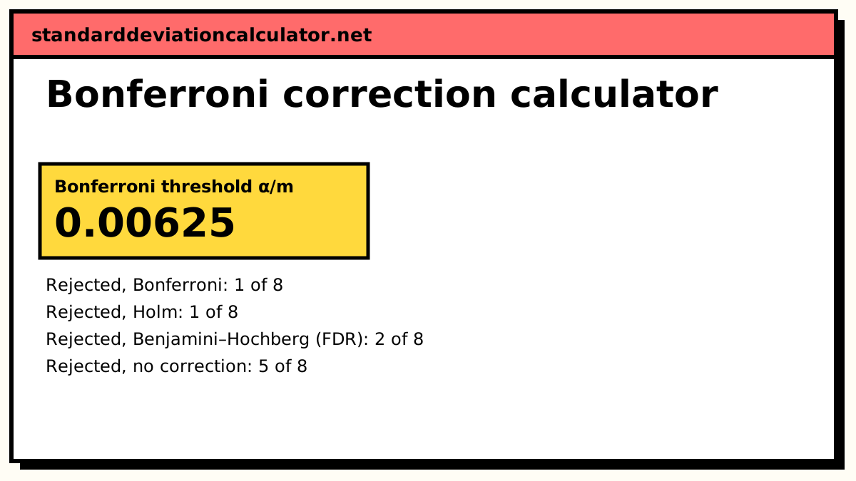
- Bonferroni: the threshold is 0.05 ÷ 8 = 0.00625. Only 0.001 is below it, so one outcome is significant. Its adjusted p is 0.001 × 8 = 0.008.
- Holm: the smallest p is multiplied by 8 (0.008), the next by 7 (0.008 × 7 = 0.056). 0.056 is above 0.05, so Holm stops and also rejects one.
- Benjamini–Hochberg: the second smallest becomes 0.008 × 8/2 = 0.032, which is below 0.05, while the third, 0.039 × 8/3 = 0.104, is not. BH rejects two.
The three methods answer different questions. Bonferroni and Holm protect against making even one false claim across all eight outcomes. Benjamini–Hochberg allows that about 5% of the claims it makes may be false, and in exchange finds the second effect.
Choosing a method
Use Holm when any single false positive is costly, for example the primary outcomes of a clinical trial. It controls the same error rate as Bonferroni and always rejects at least as many hypotheses. Use Benjamini–Hochberg when you are screening many candidates and will follow up the hits, such as gene expression, many A/B metrics or feature selection. Plain Bonferroni is worth knowing because it is simple to apply by hand and easy to explain.
Common mistakes
- Setting m to the number of significant results instead of the number of tests run.
- Correcting after dropping tests that "obviously" did not work. They still count.
- Applying a correction to planned, independent research questions that were never meant as one family. The family is the set of tests behind a single claim.
- Comparing Holm-adjusted p-values with α/m. Adjusted p-values are compared with α itself.
Common questions
What is the Bonferroni correction?
A way to keep the chance of any false positive at α when you run m tests. Either compare each p-value with α/m instead of α, or multiply each p-value by m (capping at 1) and compare with α. The two give the same decisions. With 8 tests at α = 0.05 the threshold is 0.00625.
Why is the Bonferroni correction called conservative?
It guarantees the family-wise error rate is at most α whatever the dependence between the tests, and that guarantee costs power. When tests are positively correlated, or when m is large, it rejects far fewer hypotheses than it could. Holm's method has the same guarantee and is never less powerful, so there is little reason to prefer plain Bonferroni.
What is the difference between FWER and FDR?
The family-wise error rate (FWER) is the probability of at least one false positive among all the tests. The false discovery rate (FDR) is the expected proportion of false positives among the hypotheses you reject. Controlling FDR at 5% accepts that about 1 in 20 discoveries may be wrong, which suits screening many genes or metrics. Bonferroni and Holm control FWER; Benjamini–Hochberg controls FDR.
What should m be?
The number of tests in the family you are drawing conclusions from, including the ones that were not significant and the ones you are not reporting. If you ran 20 comparisons and paste only the 5 smallest p-values, enter m = 20.
What is the Šidák correction?
A slightly less strict threshold, 1 − (1 − α)^(1/m), that is exact when the tests are independent. For 8 tests at α = 0.05 it gives 0.00639 against Bonferroni's 0.00625. The difference is small unless α or m is large.
Related calculators
-
P-value calculator
p-values from z, t, chi-square and F statistics.
-
ANOVA calculator
Compare several means in one test before running pairwise comparisons.
-
A/B test calculator
Significance and sample size for conversion-rate tests.