Wilcoxon rank-sum test calculator
Compare two independent groups by ranks. Paste the two samples; the calculator ranks all values together, adds up the ranks of the first group to get W, and compares it with the value expected if both groups came from the same distribution.
The curve is the normal approximation to W under H₀. The shaded tails hold 5% of it: a W there rejects H₀ at α = 0.05.
| Value | Group | Rank |
|---|---|---|
| 1 | Method B | 1 |
| 2 | Method B | 2.5 |
| 2 | Method B | 2.5 |
| 3 | Method B | 4.5 |
| 3 | Method B | 4.5 |
| 4 | Method A | 6.5 |
| 4 | Method B | 6.5 |
| 5 | Method A | 8.5 |
| 5 | Method B | 8.5 |
| 6 | Method A | 10.5 |
| 6 | Method B | 10.5 |
| 7 | Method A | 12 |
| 8 | Method A | 13 |
| 9 | Method A | 14 |
| 12 | Method A | 15 |
Show the working, step by step
Rank all 15 values together, smallest = 1. Tied values share the average of the ranks they occupy (tie groups of size 2, 2, 2, 2, 2).
Add up the ranks in each group.
R₁ = 79.5 (Method A, n₁ = 7), R₂ = 40.5 (Method B, n₂ = 8) check: R₁ + R₂ = N(N + 1)/2 = 120
The rank-sum statistic is the rank sum of sample 1.
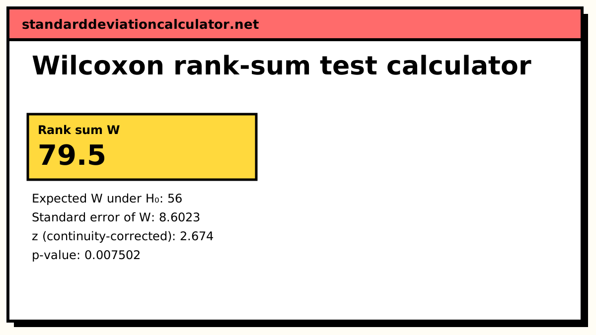
W = R₁ = 79.5
Its mean and standard error if the two groups come from the same distribution.
E(W) = n₁(N + 1)/2 = 7 × 16 / 2 = 56 SE(W) = √(n₁n₂/12 × ((N + 1) − Σ(t³ − t)/(N(N − 1)))) = √(56/12 × (16 − 30/210)) = 8.6023
Standardise W (moving it 0.5 towards the mean).
z = (W − E(W) ∓ 0.5) ÷ SE(W) = (79.5 − 56 ∓ 0.5) ÷ 8.6023 = 2.6737
p-value (two-sided), from the normal approximation with continuity correction.
p = 0.007502
W and U carry the same information: U₁ = W − n₁(n₁ + 1)/2, so the z statistic and p-value here are identical to the Mann–Whitney test.
The formulas
W = R₁ = sum of the ranks of sample 1 E(W) = n₁(N + 1) / 2 SE(W) = √[ n₁n₂/12 × ( (N + 1) − Σ(t³ − t) / (N(N − 1)) ) ] z = (W − E(W) ∓ 0.5) ÷ SE(W)
N = n₁ + n₂ and t is the size of each group of tied values. Without ties the bracket is simply N + 1. The 0.5 is a continuity correction that moves W towards its mean, because W moves in steps while the normal curve is continuous.
Worked example
Two teaching methods are tried on small classes and each student gets a quiz score out of 12. Method A: 7, 5, 6, 4, 12, 9, 8. Method B: 3, 6, 4, 2, 1, 5, 3, 2. Ranked together, the 15 scores contain five pairs of ties (2, 3, 4, 5 and 6), each pair sharing the average of two ranks.
- Ranks of method A: 12, 8.5, 10.5, 6.5, 15, 14, 13, so W = 79.5. Method B's ranks add to 40.5, and 79.5 + 40.5 = 15 × 16 ÷ 2 = 120.
- Expected W if the methods are equivalent: 7 × 16 ÷ 2 = 56.
- Standard error: √(56/12 × (16 − 30/210)) = 8.602. Each tie pair adds 2³ − 2 = 6 to the correction, 30 in all.
- z = (79.5 − 56 − 0.5) ÷ 8.602 = 2.674, two-sided p = 0.0075.
p is well below 0.05: scores under method A are systematically higher. The equivalent Mann–Whitney statistic is U₁ = 79.5 − 7 × 8 ÷ 2 = 51.5 out of a possible 56, so in 92% of A-versus-B pairs the method A student scored higher. The effect size r = 0.71 is large.
Why W and U are the same test
The smallest possible rank sum for sample 1 is 1 + 2 + … + n₁ = n₁(n₁ + 1)/2, reached when every sample 1 value is below every sample 2 value. Each time a sample 1 value moves above a sample 2 value, W rises by one and so does the count of pairs U₁. So W is U₁ plus a constant, and the mean and standard error shift by the same constant. Any conclusion from one applies to the other. Use whichever your course or journal expects, and the Mann–Whitney calculator if you need U-table critical values.
Common mistakes
- Using the test on paired measurements. Paired data need the signed-rank test.
- Forgetting the tie correction, which makes the p-value slightly too large.
- Comparing W with a U table, or U with a W table. They differ by n₁(n₁ + 1)/2.
- Treating a significant result as proof that the means differ. The test is about the ordering of values, not the means.
Common questions
Is the Wilcoxon rank-sum test the same as the Mann–Whitney U test?
Yes. Wilcoxon (1945) framed it as a sum of ranks W; Mann and Whitney (1947) framed it as a count U of pairs. They are linked by U₁ = W − n₁(n₁ + 1)/2, so they have the same z statistic and p-value. That is why software often calls it the Wilcoxon–Mann–Whitney test, and why R's wilcox.test prints "W" but reports the value of U₁.
What is the difference between the rank-sum and signed-rank tests?
The rank-sum test compares two independent groups. The Wilcoxon signed-rank test is for paired data, such as the same people before and after, and ranks the absolute differences within each pair. Using the rank-sum test on paired data throws away the pairing and loses power.
Which sample should be sample 1?
Either. Swapping the samples replaces W by the other group's rank sum and flips the sign of z, but the two-sided p-value does not change. For a one-sided test, choose the direction relative to sample 1: "sample 1 tends to be larger" or "smaller".
How do ties affect the test?
Tied values share the average of the ranks they cover, which leaves the expected W unchanged but reduces its variance. The calculator applies the standard tie correction to the standard error; in the example it lowers SE(W) from 8.641 to 8.602. With ties the exact distribution no longer applies, so the p-value comes from the normal approximation.
How large must the samples be for the normal approximation?
It is usually adequate once both groups have about 8 or more values, and it improves with the continuity correction. For smaller groups without ties the calculator uses the exact distribution, which is correct at any size.
Related calculators
-
Mann–Whitney U test
The same test written in terms of U, with exact p-values.
-
t-test calculator
Compare two means when the data are roughly normal.
-
Median calculator
Describe each group with its median before testing.