Power analysis calculator
Work out how many observations a study needs before you collect them. Choose the test, the effect size, α and the power you want, and the calculator returns the sample size, or switch to solving for the power of a sample you already have. The curve shows how power grows with n.
0.2 small, 0.5 medium, 0.8 large.
0.1 small, 0.3 medium, 0.5 large.
As a decimal: 0.8 for 80%.
━ Power of the two-sample t-test, d = 0.5
Show the working, step by step
Degrees of freedom and noncentrality for n = 64 per group.
df = 2n − 2 = 126, δ = d × √(n/2) = 0.5 × √(64/2) = 2.8284
Critical t for α = 0.05 (two-tailed).
t_crit = 1.979
Power is the chance a noncentral t with that δ lands beyond the critical value.
power = P(T′(126, 2.828) > 1.979) + P(T′ < −1.979) = 0.8015
n is the smallest whole number that reaches 80% power, so the achieved power is slightly above the target.
The four quantities
Power analysis links four numbers: the effect size, the significance level α, the power 1 − β and the sample size n. Fix any three and the fourth follows. Most often α = 0.05 and power = 0.80 are set by convention, the effect size comes from subject knowledge, and n is the unknown.
The formulas
Two-sample t: df = 2n − 2, δ = d √(n/2) One-sample / paired t: df = n − 1, δ = d √n power = P(T′(df, δ) > t_crit) + P(T′(df, δ) < −t_crit)
T′ is a noncentral t variable: the distribution the t statistic follows when the true standardised difference is d. The calculator evaluates it exactly and searches for the smallest n that reaches the target. For proportions and correlations it uses closed forms:
Proportions: n = [z_α √(2p̄(1 − p̄)) + z_β √(p₁(1 − p₁) + p₂(1 − p₂))]² ÷ (p₁ − p₂)² Correlation: n = ((z_α + z_β) ÷ atanh r)² + 3
z_α is z₀.₀₂₅ = 1.960 for a two-tailed test at 5%, and z_β is z₀.₂₀ = 0.842 for 80% power.
Worked example
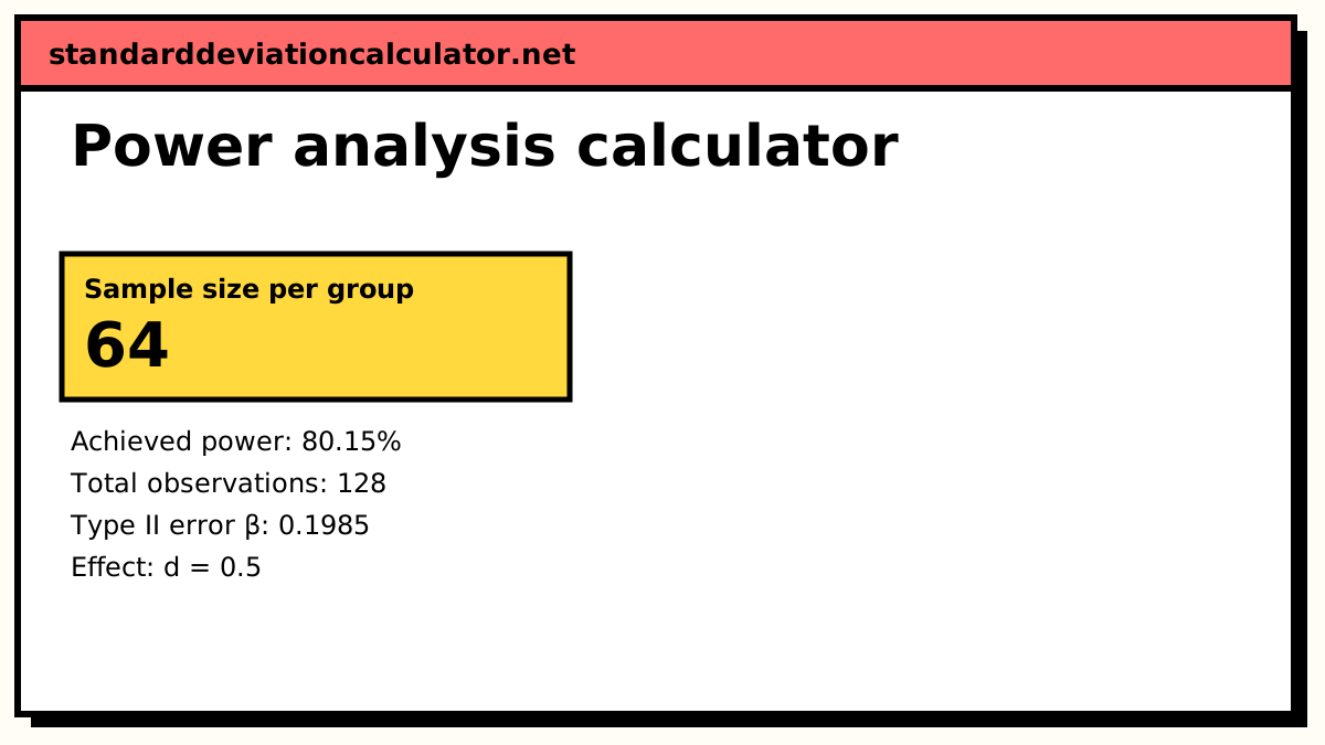
A trial will compare a new teaching method with the current one. The smallest improvement worth detecting is half a standard deviation, d = 0.5. With α = 0.05 two-tailed and 80% power:
- Try n = 64 per group: df = 126, δ = 0.5 × √32 = 2.828, and t_crit = 1.979.
- The chance that T′(126, 2.828) exceeds 1.979 is 0.8015, so power is 80.15%.
- At n = 63 power is 79.5%, just short. The answer is 64 per group, 128 in total.
The normal shortcut 2(1.960 + 0.842)² ÷ 0.5² = 62.8 gives 63, one fewer, because it ignores the extra uncertainty from estimating the standard deviation. For the other designs with the default settings: a one-sample or paired t-test with d = 0.5 needs 34 subjects, comparing 10% with 15% needs 686 per group, and detecting r = 0.3 needs 85 cases.
Reading the power curve
Power rises steeply at first and then flattens as it approaches 1. Moving from 80% to 90% power for d = 0.5 takes 86 per group instead of 64, about a third more. Halving the effect size to d = 0.25 roughly quadruples the sample, because n grows with 1/d².
Common mistakes
- Using an optimistic effect size from a small pilot study, which tends to overstate effects.
- Forgetting drop-out. If you expect 15% to leave the study, divide n by 0.85.
- Planning with a two-sample formula for a paired design, or the reverse. Pairing usually needs far fewer subjects.
- Computing "observed power" after a non-significant result as if it explained the result.
Common questions
What is statistical power?
The probability that a test rejects H₀ when a real effect of the stated size exists. Power is 1 − β, where β is the chance of a false negative. A study with 50% power misses a real effect half the time, so a non-significant result from it says very little.
What effect size should I use?
The smallest effect that would matter in practice, not the effect you hope to see. Take it from earlier studies, a pilot, or a judgement of what difference is worth acting on. Cohen's labels (d = 0.2, 0.5, 0.8; r = 0.1, 0.3, 0.5) are a last resort when nothing better exists. Overestimating the effect is the most common reason studies turn out underpowered.
How accurate are the numbers?
For t-tests the calculator uses the exact noncentral t distribution (algorithm AS 243), so the results match G*Power and R's pwr package: 64 per group for d = 0.5 at 80% power. For two proportions it uses the normal approximation with the pooled standard error under H₀, and for correlations Fisher's z transformation, which can be one or two above the exact answer.
Is the sample size per group or in total?
For the two-sample t-test and two proportions the answer is per group, with equal group sizes. Double it for the total. For the one-sample or paired t-test it is the number of subjects or pairs, and for a correlation the number of cases.
Should I calculate power after the study is done?
Not with the observed effect size. "Observed power" is a direct function of the p-value and adds no information. Power is a planning tool. After the study, report the confidence interval, which shows which effect sizes the data rule out.
Related calculators
-
Sample size calculator
Sample size to estimate a mean or proportion to a set margin of error.
-
Cohen's d calculator
Compute the standardised effect size from means and SDs.
-
A/B test calculator
Plan and analyse conversion-rate experiments.