Hypothesis testing calculator
Test a claim about a population mean or proportion. Enter the sample summary, pick the alternative hypothesis and α, and the calculator states H₀ and H₁, computes the test statistic, p-value and critical value, and writes the conclusion in plain English.
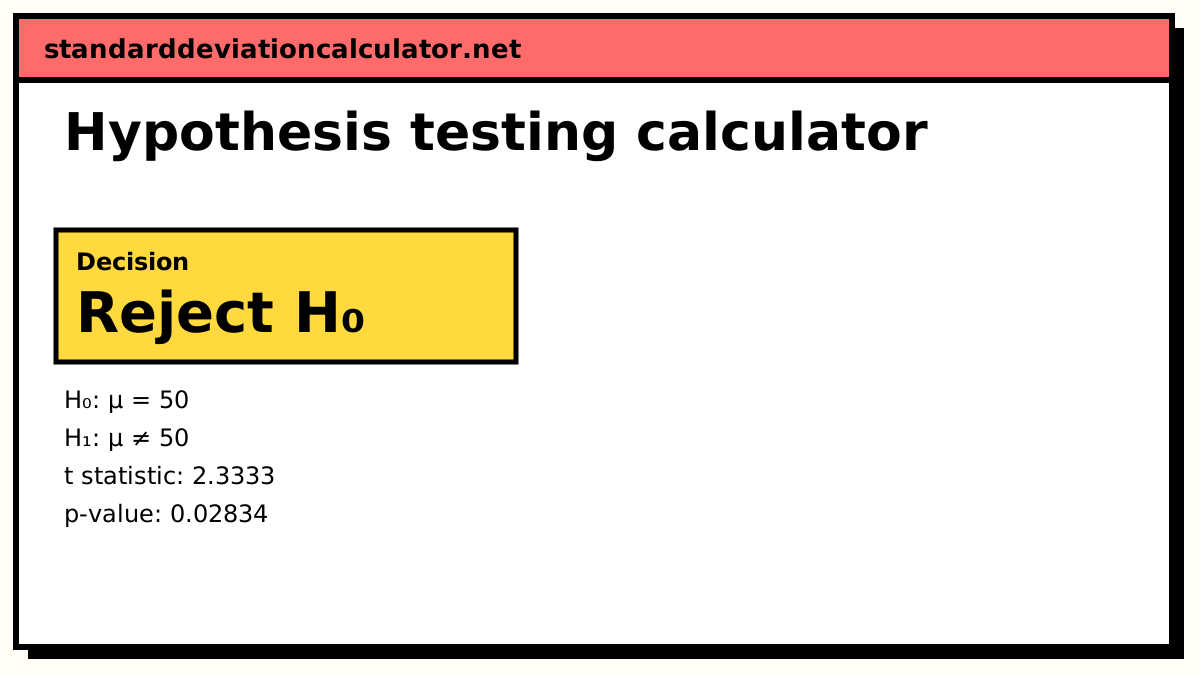
Conclusion. At the 0.05 significance level there is enough evidence to conclude that the population mean differs from 50 (p = 0.02834).
Shaded: rejection region (total area α = 0.05). Dot: your t statistic.
Show the working, step by step
Standard error of the mean.
SE = s ÷ √n = 4.5 ÷ √25 = 0.9
Test statistic, with df = n − 1 = 24.
t = (x̄ − μ₀) ÷ SE = (52.1 − 50) ÷ 0.9 = 2.3333
p-value for H₁: μ ≠ 50.
p = 2 × P(T(24) > |2.3333|) = 0.02834
Critical value at α = 0.05: reject H₀ when |t| > 2.064.
2.333 is in the rejection region, and p = 0.02834 < 0.05: reject H₀.
The p-value and the critical-value methods always agree: the statistic falls in the shaded region exactly when p is below α.
The formulas
t = (x̄ − μ₀) ÷ (s / √n), df = n − 1 z = (x̄ − μ₀) ÷ (σ / √n) z = (p̂ − p₀) ÷ √(p₀(1 − p₀) / n)
Each statistic measures how many standard errors the sample result sits from the value claimed by the null hypothesis. The proportion test uses p₀ in the standard error, not p̂, because the calculation assumes H₀ is true.
The five steps of a hypothesis test
- State the hypotheses. H₀ gives a single value (μ = 50); H₁ says the parameter is different, smaller or larger.
- Choose α, the risk of rejecting a true H₀ you will accept. 0.05 is the convention, not a law.
- Compute the test statistic from the sample.
- Find the p-value, or compare the statistic with the critical value.
- Decide, and state the conclusion in the language of the problem.
Worked example
A bottling line should fill cartons with 50 ml of concentrate on average. A sample of 25 cartons has mean x̄ = 52.1 ml and standard deviation s = 4.5 ml. Is the machine off target? The standard deviation comes from the sample, so this is a t-test with 24 degrees of freedom.
- H₀: μ = 50, H₁: μ ≠ 50 (two-tailed), α = 0.05.
- Standard error: 4.5 ÷ √25 = 0.9.
- Test statistic: t = (52.1 − 50) ÷ 0.9 = 2.333.
- p-value: 2 × P(T₂₄ > 2.333) = 0.0283.
- Critical value: t₀.₀₂₅,₂₄ = 2.064, so the rejection region is |t| > 2.064.
2.333 is beyond 2.064 and 0.0283 is below 0.05, so both methods reject H₀. In words: at the 5% level there is enough evidence that the mean fill differs from 50 ml. The chart shows the t curve with both tails shaded; the statistic sits inside the right-hand shaded area.
At α = 0.01 the critical value rises to 2.797 and the same data no longer reject H₀. That is why α has to be fixed before looking at the result.
Interpreting the result
The p-value is the probability, assuming H₀ is true, of a statistic at least as far from the null value as the one observed. It is not the probability that H₀ is true, and 1 − p is not the probability that H₁ is true. A small p-value says the data would be surprising if H₀ held.
Statistical significance is also not practical importance. With thousands of observations a difference of 0.1 ml can be significant and still not worth fixing. Report the size of the difference, here 2.1 ml, next to the p-value.
Common mistakes
- Using the z-test with a sample standard deviation. Unless σ is genuinely known, use t.
- Picking a one-tailed test after seeing which way the data went.
- Writing "accept H₀". The correct wording is "do not reject H₀".
- Using p̂ instead of p₀ in the standard error of the proportion test.
- Running a one-sample test on paired or two-group data. Paired data need differences first; two groups need a two-sample test.
Common questions
How do I choose between the z-test and the t-test for a mean?
Use the t-test when the standard deviation comes from your sample, which is almost always. The z-test is for the rare case where the population standard deviation σ is known in advance, for example from a long-running manufacturing process. With large samples the two give nearly the same answer; with small samples the t-test's wider tails matter.
What is the difference between the p-value and the critical value approach?
They are two views of the same decision. The critical value approach asks whether the test statistic falls in the rejection region (beyond ±2.064 in the default example). The p-value approach asks whether the probability of a result at least this extreme is below α. One says reject exactly when the other does.
When should I use a one-tailed test?
Only when the direction was fixed before you saw the data and a result in the other direction would lead to the same action as no result. A one-tailed test puts all of α in one tail, so it halves the p-value for results in the predicted direction. Choosing the tail after looking at the data doubles the real false-positive rate.
Does "do not reject H₀" mean H₀ is true?
No. It means the data are not inconsistent with H₀ at the chosen level. A small sample can fail to detect a real difference. To say something positive about a small effect, look at a confidence interval or run a power analysis before collecting data.
What conditions does the proportion test need?
A random sample, independent observations, and at least 10 expected successes and 10 expected failures under H₀ (np₀ ≥ 10 and n(1 − p₀) ≥ 10). The calculator warns when these fail. For smaller samples use an exact binomial test.
Related calculators
-
t-test calculator
One-sample, two-sample and paired t-tests from raw data.
-
P-value calculator
p-values from z, t, chi-square and F statistics.
-
Power analysis calculator
Sample size and power for t-tests, proportions and correlations.