Mann–Whitney U test calculator
Compare two independent groups without assuming normal data. Paste the two samples; the calculator ranks them together, computes U for each group and gives the exact or approximate p-value, with every rank shown.
Bars: P(U₁ = k) if H₀ is true. Solid bars: the rejection region at α = 0.05 (two-sided). The observed U₁ falls outside it, so H₀ is not rejected.
| Value | Group | Rank |
|---|---|---|
| 0.73 | At term | 1 |
| 0.74 | 12–26 weeks | 2 |
| 0.8 | At term | 3 |
| 0.83 | At term | 4 |
| 0.88 | 12–26 weeks | 5 |
| 0.9 | 12–26 weeks | 6 |
| 1.04 | At term | 7 |
| 1.15 | 12–26 weeks | 8 |
| 1.21 | 12–26 weeks | 9 |
| 1.38 | At term | 10 |
| 1.45 | At term | 11 |
| 1.46 | At term | 12 |
| 1.64 | At term | 13 |
| 1.89 | At term | 14 |
| 1.91 | At term | 15 |
Show the working, step by step
Rank all 15 values together, smallest = 1. Tied values share the average of the ranks they occupy.
Add up the ranks in each group.
R₁ = 90 (At term, n₁ = 10), R₂ = 30 (12–26 weeks, n₂ = 5) check: R₁ + R₂ = N(N + 1)/2 = 120
Convert rank sums to U.
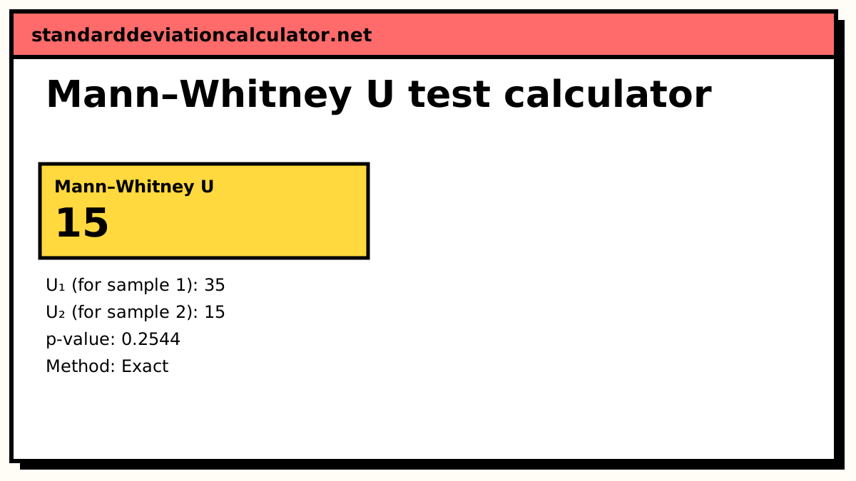
U₁ = R₁ − n₁(n₁ + 1)/2 = 90 − 55 = 35 U₂ = n₁n₂ − U₁ = 50 − 35 = 15 U = min(U₁, U₂) = 15
Mean and standard deviation of U under H₀.
μ_U = n₁n₂/2 = 25 σ_U = √(n₁n₂/12 × ((N + 1) − Σ(t³ − t)/(N(N − 1)))) = 8.165
Standardise U₁ (moving it 0.5 towards the mean).
z = (U₁ − μ_U ∓ 0.5) ÷ σ_U = 1.1635
p-value (two-sided), from the exact distribution of U (no ties, both n ≤ 20).
exact p = 0.2544 (normal approximation: 0.2446)
U₁ counts, over all n₁n₂ pairs, how often a value from sample 1 beats one from sample 2 (ties count ½). Some books report U = min(U₁, U₂) and compare it with a lower critical value; the p-value is the same.
The formulas
U₁ = R₁ − n₁(n₁ + 1)/2, U₂ = n₁n₂ − U₁ μ_U = n₁n₂/2 σ_U = √[ n₁n₂/12 × ( (N + 1) − Σ(t³ − t) / (N(N − 1)) ) ] z = (U₁ − μ_U ∓ 0.5) ÷ σ_U
R₁ is the sum of the ranks of sample 1 in the combined data, N = n₁ + n₂, and t is the size of each group of tied values. U₁ also has a direct meaning: over all n₁n₂ pairs of one value from each group, it counts how many times the sample 1 value is larger, with ties counting ½.
Worked example
The default data are permeability measurements of the membrane around a fetus: 10 at full term and 5 taken between 12 and 26 weeks of pregnancy (the example in R's wilcox.test help page). Ranked together, the term values receive ranks 1, 3, 4, 7, 10, 11, 12, 13, 14 and 15.
- Rank sums: R₁ = 90 for the term group and R₂ = 30 for the early group. Check: 90 + 30 = 15 × 16 ÷ 2 = 120.
- U₁ = 90 − 10 × 11 ÷ 2 = 35, U₂ = 10 × 5 − 35 = 15, so U = 15.
- There are no ties and both groups are small, so the p-value is exact. Of the C(15, 5) = 3,003 equally likely ways to assign the ranks, 382 give U₁ ≥ 35, a one-tailed probability of 0.1272. Doubling gives the two-tailed p = 0.2544.
- The normal approximation would give z = 1.16 and p = 0.245, close to the exact value.
From a table, the two-tailed 5% critical value for n₁ = 10 and n₂ = 5 is 8. U = 15 is above it, and p = 0.25 is above 0.05, so the difference between the groups is not significant. The term values tend to be higher (P(term > early) = 35 ÷ 50 = 0.70), but with only five early measurements that could easily be chance.
Assumptions
- The two samples are independent of each other. For paired data use the Wilcoxon signed-rank test.
- Observations within each group are independent.
- The variable is at least ordinal, so the values can be put in order.
Normality is not required. That is the reason to choose this test, not a weakness of it.
Common mistakes
- Ranking each group separately. The ranks must come from the combined data.
- Giving tied values different ranks. Ties share the average of the ranks they span.
- Comparing U₁ with a lower-tail table value. Tables expect the smaller of U₁ and U₂.
- Reporting the result as "the medians differ" when the two distributions have different shapes.
Common questions
When should I use the Mann–Whitney U test instead of a t-test?
When you are comparing two independent groups and the data are ordinal (ratings, ranks) or clearly non-normal with small samples, for example strongly skewed times or incomes with outliers. The test uses only the order of the values, so a single extreme value cannot drag the result around. With roughly normal data the t-test is slightly more powerful.
Does the Mann–Whitney test compare medians?
Only if the two distributions have the same shape and differ just by a shift. In general it tests whether a value from one group tends to be larger than a value from the other, that is, whether P(X > Y) differs from ½. Two groups can have equal medians and still give a significant result if their shapes differ.
Which U do I report, U₁, U₂ or the smaller one?
Any of them, as long as you say which. U₁ + U₂ = n₁n₂, so one determines the other. Printed critical-value tables use the smaller U and reject when it is at or below the table value. R and most software report U₁ (called W in R's output). The p-value is the same either way.
When is the exact p-value used?
When there are no tied values and both groups have at most 20 observations. The calculator then counts, among all C(n₁ + n₂, n₁) equally likely ways to split the ranks, how many give a U at least as extreme. With ties or larger groups it uses the normal approximation with the tie and continuity corrections, as R's wilcox.test does.
What effect size goes with the Mann–Whitney test?
Two are common. r = |z| ÷ √N, read with the usual 0.1 / 0.3 / 0.5 benchmarks, and the common-language effect size U₁ ÷ (n₁n₂), the probability that a random value from group 1 beats one from group 2. In the example that probability is 35 ÷ 50 = 0.70.
Related calculators
-
Wilcoxon rank-sum test
The same test written as a rank sum W, with its mean and standard error.
-
t-test calculator
The parametric comparison of two means.
-
Spearman's rank correlation
Another rank-based method, for association between two variables.