Statistics
Marshall–Edgeworth price index calculator
The Marshall–Edgeworth index weights each price by the quantity bought in both years together, q₀ + q₁. Enter base and current prices and quantities for each commodity.
Add a row for each commodity. Prices must be above zero; quantities and weights cannot be negative.
| Commodity | p₀ | q₀ | p₁ | q₁ | p₀q₀ | p₁q₀ | p₀q₁ | p₁q₁ |
|---|---|---|---|---|---|---|---|---|
| A | 10 | 20 | 15 | 15 | 200 | 300 | 150 | 225 |
| B | 8 | 15 | 10 | 14 | 120 | 150 | 112 | 140 |
| C | 5 | 30 | 6 | 36 | 150 | 180 | 180 | 216 |
| D | 20 | 10 | 24 | 9 | 200 | 240 | 180 | 216 |
| E | 4 | 25 | 4 | 32 | 100 | 100 | 128 | 128 |
| Σ | 770 | 970 | 750 | 925 |
Pale bars: each commodity on its own. Solid bar: the Marshall–Edgeworth index, which weights them together. The dashed line is the base, 100; above it means prices rose.
Show the working, step by step
Multiply across each row to get p₀q₀, p₁q₀, p₀q₁, p₁q₁, then add each column.
Σp₀q₀ = 770 Σp₁q₀ = 970 Σp₀q₁ = 750 Σp₁q₁ = 925
Add the base-weighted and current-weighted totals: Σp(q₀ + q₁) = Σpq₀ + Σpq₁.
Σp₁(q₀ + q₁) = 970 + 925 = 1895 Σp₀(q₀ + q₁) = 770 + 750 = 1520
Divide and multiply by 100.
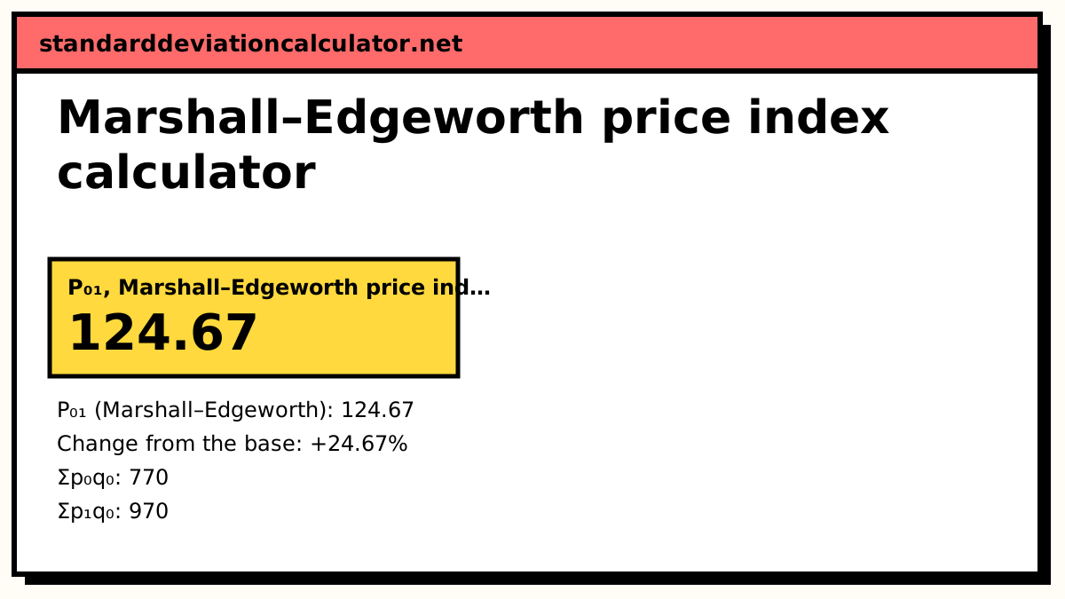
P₀₁ (Marshall–Edgeworth) = 1895 / 1520 × 100 = 124.67
P₀₁ = 124.67 means prices in the current period are 24.67% higher than in the base period. Time reversal test: P₁₀ = 80.21, and P₀₁ × P₁₀ = 124.67/100 × 80.21/100 = 1.0000, which equals 1, so the test is met.
The formula
P₀₁ = Σp₁(q₀ + q₁) / Σp₀(q₀ + q₁) × 100 = (Σp₁q₀ + Σp₁q₁) / (Σp₀q₀ + Σp₀q₁) × 100
Alfred Marshall and Francis Edgeworth suggested it in the 1880s as a middle way between Laspeyres (weights q₀) and Paasche (weights q₁). Using the sum of the two baskets means neither year's buying pattern decides the weights alone. The second line is how it is usually worked in exams: compute the four products once and add them in pairs.
A worked example
The calculator's default data:
| Commodity | p₀ | q₀ | p₁ | q₁ | p₀q₀ | p₁q₀ | p₀q₁ | p₁q₁ |
|---|---|---|---|---|---|---|---|---|
| A | 10 | 20 | 15 | 15 | 200 | 300 | 150 | 225 |
| B | 8 | 15 | 10 | 14 | 120 | 150 | 112 | 140 |
| C | 5 | 30 | 6 | 36 | 150 | 180 | 180 | 216 |
| D | 20 | 10 | 24 | 9 | 200 | 240 | 180 | 216 |
| E | 4 | 25 | 4 | 32 | 100 | 100 | 128 | 128 |
| Σ | 770 | 970 | 750 | 925 |
- Numerator: Σp₁q₀ + Σp₁q₁ = 970 + 925 = 1,895.
- Denominator: Σp₀q₀ + Σp₀q₁ = 770 + 750 = 1,520.
- P₀₁ = 1,895 / 1,520 × 100 = 124.67.
Prices rose by 24.67% on this measure, between the Laspeyres figure of 125.97 and the Paasche figure of 123.33.
Does it over- or under-state inflation?
Much less than either parent formula. Laspeyres overstates the rise in the cost of living because it ignores substitution away from dearer goods; Paasche understates it because its basket has already substituted. Marshall–Edgeworth blends the two baskets, so the upward and downward substitution biases largely cancel. It always lies between L and P, because (a + c) / (b + d) sits between a / b and c / d, and it tracks Fisher's ideal index closely (124.65 here). What it still misses, like every fixed-formula index, is new goods and quality change.
Tests it passes
| Test | Result | Default example |
|---|---|---|
| Time reversal (P₀₁ × P₁₀ = 1) | Passes | 1.2467 × 0.8021 = 1.0000 |
| Factor reversal (P₀₁ × Q₀₁ = V₀₁) | Fails | 1.2001 against V₀₁ = 1.2013 |
Common mistakes
- Averaging Laspeyres and Paasche and calling it Marshall–Edgeworth. That is the Dorbish–Bowley index (124.65 here). The two are close but they are different formulas.
- Adding prices instead of values: the formula adds p × (q₀ + q₁), not p₀ + p₁.
Common questions
What is the Marshall–Edgeworth price index formula?
P₀₁ = Σp₁(q₀ + q₁) / Σp₀(q₀ + q₁) × 100, which expands to
(Σp₁q₀ + Σp₁q₁) / (Σp₀q₀ + Σp₀q₁) × 100. The weight for each commodity is the
total quantity bought across the two years. For the default data it is (970 + 925) / (770 +
750) × 100 = 1895 / 1520 × 100 = 124.67.
Does the Marshall–Edgeworth index satisfy the time reversal test?
Yes. Swapping the years swaps numerator and denominator (q₀ + q₁ is the same either way round), so P₁₀ = 1520 / 1895 × 100 = 80.21 and P₀₁ × P₁₀ = 1. It fails the factor reversal test: P₀₁ × Q₀₁ = 1.2467 × 0.9626 = 1.2001, while the value ratio V₀₁ is 1.2013.
Is Marshall–Edgeworth the same as Kelly’s index?
Kelly's index with the average quantity (q₀ + q₁)/2 as its fixed weight gives exactly the Marshall–Edgeworth answer, because the ½ cancels top and bottom. Kelly's method is more general: its fixed quantities can come from any period or survey.
Is Marshall–Edgeworth close to Fisher’s index?
Usually very close. On the default data it gives 124.67 against Fisher's 124.65. Both sit between Laspeyres (125.97) and Paasche (123.33). Marshall–Edgeworth is easier to work by hand because it needs no square root, which is why it appears often in exams.
What is its main weakness?
Adding quantities from two periods lets a large country or a large shop dominate when comparing two very different places or sizes. For international comparisons this makes the index lean towards the bigger economy's pattern of prices.
Related calculators
-
Laspeyres price index
Base-year quantities as weights.
-
Paasche price index
Current-year quantities as weights.
-
Kelly’s price index
Any fixed basket q; with q = (q₀ + q₁)/2 it equals Marshall–Edgeworth.
-
Fisher’s ideal index
Passes both the time and factor reversal tests.
-
Weighted aggregative index
All six weighted methods on the same data.