Statistics
Fisher’s ideal index calculator
Fisher's ideal index is the geometric mean of the Laspeyres and Paasche indices. Enter base and current prices and quantities; the calculator shows L, P, the Fisher index and both reversal tests with your numbers substituted.
Add a row for each commodity. Prices must be above zero; quantities and weights cannot be negative.
Dorbish–Bowley is the arithmetic mean of Laspeyres and Paasche; Fisher is their geometric mean, so it is never larger.
| Commodity | p₀ | q₀ | p₁ | q₁ | p₀q₀ | p₁q₀ | p₀q₁ | p₁q₁ |
|---|---|---|---|---|---|---|---|---|
| A | 10 | 20 | 15 | 15 | 200 | 300 | 150 | 225 |
| B | 8 | 15 | 10 | 14 | 120 | 150 | 112 | 140 |
| C | 5 | 30 | 6 | 36 | 150 | 180 | 180 | 216 |
| D | 20 | 10 | 24 | 9 | 200 | 240 | 180 | 216 |
| E | 4 | 25 | 4 | 32 | 100 | 100 | 128 | 128 |
| Σ | 770 | 970 | 750 | 925 |
Show the working, step by step
Multiply across each row to get p₀q₀, p₁q₀, p₀q₁, p₁q₁, then add each column.
Σp₀q₀ = 770 Σp₁q₀ = 970 Σp₀q₁ = 750 Σp₁q₁ = 925
Laspeyres and Paasche indices:
L = Σp₁q₀ / Σp₀q₀ × 100 = 970 / 770 × 100 = 125.97 P = Σp₁q₁ / Σp₀q₁ × 100 = 925 / 750 × 100 = 123.33
Take their geometric mean.
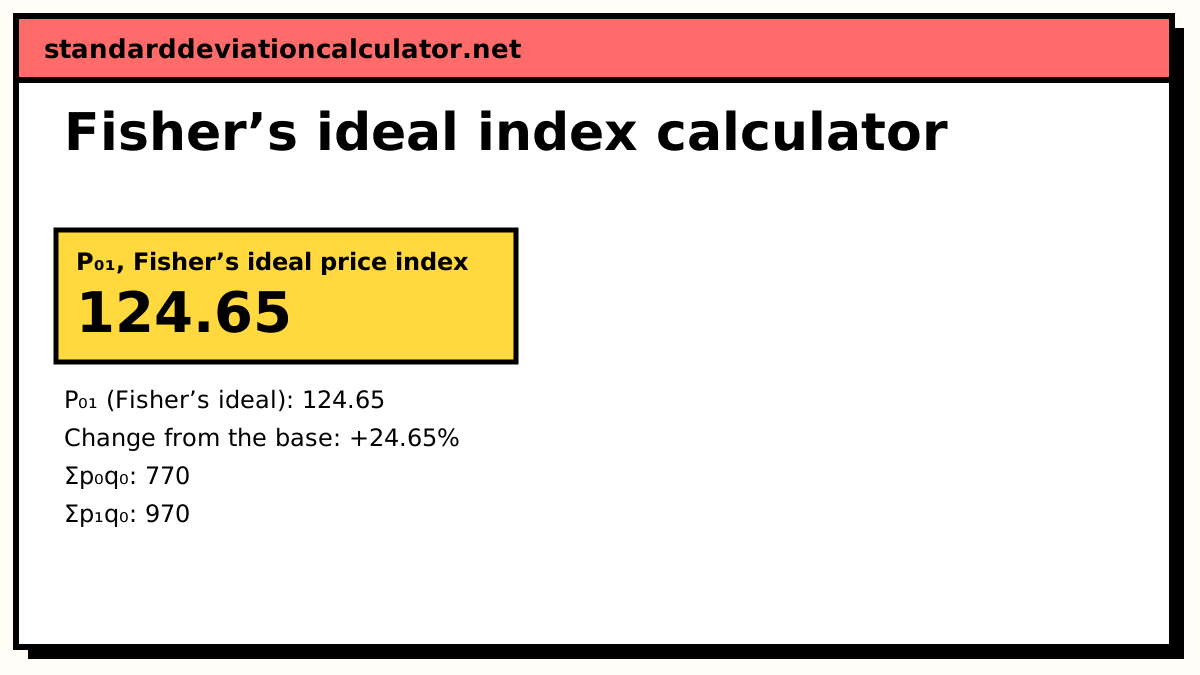
P₀₁ (Fisher) = √(L × P) = √(1.25974 × 1.23333) × 100 = 124.65
P₀₁ = 124.65 means prices in the current period are 24.65% higher than in the base period. Time reversal test: P₁₀ = 80.23, and P₀₁ × P₁₀ = 124.65/100 × 80.23/100 = 1.0000, which equals 1, so the test is met.
Time reversal test: P₀₁ × P₁₀ = 1
P₁₀ = √(Σp₀q₁/Σp₁q₁ × Σp₀q₀/Σp₁q₀) × 100 = √(750/925 × 770/970) × 100 = 80.23 P₀₁ × P₁₀ = 1.24647 × 0.802268 = 1.0000 ✓ met
Factor reversal test: P₀₁ × Q₀₁ = V₀₁
Q₀₁ = √(Σq₁p₀/Σq₀p₀ × Σq₁p₁/Σq₀p₁) × 100 = √(750/770 × 925/970) × 100 = 96.38 P₀₁ × Q₀₁ = 1.24647 × 0.963763 = 1.2013 V₀₁ = Σp₁q₁ / Σp₀q₀ = 925 / 770 = 1.2013 ✓ met
The formula
P₀₁ = √( Σp₁q₀/Σp₀q₀ × Σp₁q₁/Σp₀q₁ ) × 100 = √(L × P)
Work out the four aggregates Σp₀q₀, Σp₁q₀, Σp₀q₁ and Σp₁q₁, form the Laspeyres and Paasche ratios, multiply them and take the square root. The quantity index has the same shape with p and q swapped:
Q₀₁ = √( Σq₁p₀/Σq₀p₀ × Σq₁p₁/Σq₀p₁ ) × 100
A worked example
The calculator's default data:
| Commodity | p₀ | q₀ | p₁ | q₁ | p₀q₀ | p₁q₀ | p₀q₁ | p₁q₁ |
|---|---|---|---|---|---|---|---|---|
| A | 10 | 20 | 15 | 15 | 200 | 300 | 150 | 225 |
| B | 8 | 15 | 10 | 14 | 120 | 150 | 112 | 140 |
| C | 5 | 30 | 6 | 36 | 150 | 180 | 180 | 216 |
| D | 20 | 10 | 24 | 9 | 200 | 240 | 180 | 216 |
| E | 4 | 25 | 4 | 32 | 100 | 100 | 128 | 128 |
| Σ | 770 | 970 | 750 | 925 |
- L = 970 / 770 = 1.25974, P = 925 / 750 = 1.23333.
- P₀₁ = √(1.25974 × 1.23333) × 100 = √1.55368 × 100 = 124.65.
Time reversal test
P₁₀ = √(Σp₀q₁/Σp₁q₁ × Σp₀q₀/Σp₁q₀) = √(750/925 × 770/970) = 0.80227 P₀₁ × P₁₀ = 1.24647 × 0.80227 = 1.0000 ✓
Factor reversal test
Q₀₁ = √(Σq₁p₀/Σq₀p₀ × Σq₁p₁/Σq₀p₁) = √(750/770 × 925/970) = 0.96376 P₀₁ × Q₀₁ = 1.24647 × 0.96376 = 1.2013 V₀₁ = Σp₁q₁ / Σp₀q₀ = 925 / 770 = 1.2013 ✓
Total spending rose by 20.13%. Fisher splits that exactly into a price change (+24.65%) and a quantity change (−3.62%): 1.24647 × 0.96376 = 1.2013. Laspeyres cannot do this: its price and quantity indices multiply to 1.2597 × 0.9740 = 1.2270, which overstates the change in value.
Why it is called “ideal”
Irving Fisher judged index formulas by whether they behave consistently. An index that says prices rose 25% from 2020 to 2025 should say they fell back by the same factor from 2025 to 2020 (time reversal), and the price index times the quantity index should give the actual change in spending (factor reversal). Laspeyres, Paasche and Dorbish–Bowley fail both; Marshall–Edgeworth and Kelly pass only time reversal. Fisher's formula passes both, which is the reason for the name and the reason it is the favourite of exam questions on the tests.
Does it over- or under-state inflation?
Laspeyres overstates the cost-of-living change (it ignores substitution away from goods that became dear) and Paasche understates it (its basket has already substituted). The geometric mean of the two sits between them, and economic theory shows that for common patterns of consumer behaviour it is very close to the true cost-of-living index. Fisher is therefore close to unbiased with respect to substitution. It still needs current quantities, so in practice it is published later than a Laspeyres CPI, and like every formula it cannot correct for new goods or quality changes by itself.
Common mistakes
- Averaging L and P arithmetically. (L + P) / 2 is the Dorbish–Bowley index; Fisher is the geometric mean √(L × P). The two are close but only Fisher passes the reversal tests.
- Rounding too early. Keep L and P to four or five decimals as ratios (1.25974, not 1.26) before multiplying, or the reversal tests will not come out to exactly 1 and V₀₁.
- Using Laspeyres in the factor reversal check. Only the Fisher Q₀₁ makes the product equal V₀₁.
Common questions
What is the formula for Fisher’s ideal index?
P₀₁ = √(Σp₁q₀/Σp₀q₀ × Σp₁q₁/Σp₀q₁) × 100 = √(L × P), the geometric
mean of the Laspeyres and Paasche indices. For the default data,
√(1.25974 × 1.23333) × 100 = 124.65.
Why is Fisher’s index called “ideal”?
Irving Fisher (The Making of Index Numbers, 1922) tested well over a hundred formulas and called this one ideal because it passes both of his reversal tests: the time reversal test (P₀₁ × P₁₀ = 1) and the factor reversal test (P₀₁ × Q₀₁ = V₀₁). It also uses both years' quantities, so it is free of the one-sided weighting of Laspeyres and Paasche, and it lies between them. It does not pass every test (it fails the circular test), so “ideal” is relative to the tests of its time.
How do you prove Fisher’s index satisfies the time reversal test?
Swap 0 and 1: P₁₀ = √(Σp₀q₁/Σp₁q₁ × Σp₀q₀/Σp₁q₀). Multiply by P₀₁ and every
sum cancels: P₀₁ × P₁₀ = √(1) = 1. With the default data, P₁₀ = √(750/925 × 770/970) × 100
= 80.23, and 1.24647 × 0.80227 = 1.0000.
How do you prove the factor reversal test for Fisher’s index?
Swap p and q to get the quantity index Q₀₁ = √(Σq₁p₀/Σq₀p₀ × Σq₁p₁/Σq₀p₁).
In P₀₁ × Q₀₁, Σp₁q₀ and Σp₀q₁ cancel and what is left is √((Σp₁q₁)² / (Σp₀q₀)²) = Σp₁q₁ / Σp₀q₀
= V₀₁. On the default data Q₀₁ = 96.38, and 1.24647 × 0.96376 = 1.2013 = 925 / 770.
Is Fisher’s index used in practice?
Yes. The US personal consumption expenditures (PCE) price index and the US GDP price measures are chain-type Fisher indices, and the IMF's CPI manual lists Fisher among the “superlative” indices that approximate a true cost-of-living index. Consumer price indices themselves are mostly Laspeyres-type, because current-period quantities arrive too late for a monthly release.
Does Fisher’s index overstate or understate inflation?
Neither in a systematic way. Laspeyres' upward substitution bias and Paasche's downward bias cancel in the geometric mean. What remains is bias from new products and quality change, which affects every formula.
Related calculators
-
Laspeyres price index
The L in √(L × P): base-year quantities as weights.
-
Paasche price index
The P in √(L × P): current-year quantities as weights.
-
Dorbish–Bowley index
The arithmetic mean of L and P instead of the geometric.
-
Weighted aggregative index
Which formulas pass which tests, on your data.
-
Geometric mean
The nth root of a product, the average behind Fisher’s formula.