Statistics
Weighted aggregative index calculator
Enter prices and quantities once and compare every weighted aggregative formula on the same data. Pick a method to see its working; the table under the result lists all six with their reversal tests.
Add a row for each commodity. Prices must be above zero; quantities and weights cannot be negative.
The solid bar is the method you chose (Laspeyres). Laspeyres and Paasche usually bracket the others; Fisher sits between them.
| Commodity | p₀ | q₀ | p₁ | q₁ | p₀q₀ | p₁q₀ |
|---|---|---|---|---|---|---|
| A | 10 | 20 | 15 | 15 | 200 | 300 |
| B | 8 | 15 | 10 | 14 | 120 | 150 |
| C | 5 | 30 | 6 | 36 | 150 | 180 |
| D | 20 | 10 | 24 | 9 | 200 | 240 |
| E | 4 | 25 | 4 | 32 | 100 | 100 |
| Σ | 770 | 970 |
| Method | Weights | P₀₁ | P₀₁ × P₁₀ | P₀₁ × Q₀₁ |
|---|---|---|---|---|
| Laspeyres | w = q₀ | 125.97 | 1.0214 ✗ | 1.2270 ✗ |
| Paasche | w = q₁ | 123.33 | 0.9790 ✗ | 1.1761 ✗ |
| Marshall–Edgeworth | w = q₀ + q₁ | 124.67 | 1.0000 ✓ | 1.2001 ✗ |
| Dorbish–Bowley | mean of L and P | 124.65 | 1.0001 ✗ | 1.2014 ✗ |
| Fisher’s ideal | geometric mean of L and P | 124.65 | 1.0000 ✓ | 1.2013 ✓ |
| Kelly’s | w = q, here (q₀ + q₁)/2 | 124.67 | 1.0000 ✓ | — |
Show the working, step by step
Multiply across each row to get p₀q₀, p₁q₀, then add each column.
Σp₀q₀ = 770 Σp₁q₀ = 970
Divide and multiply by 100.
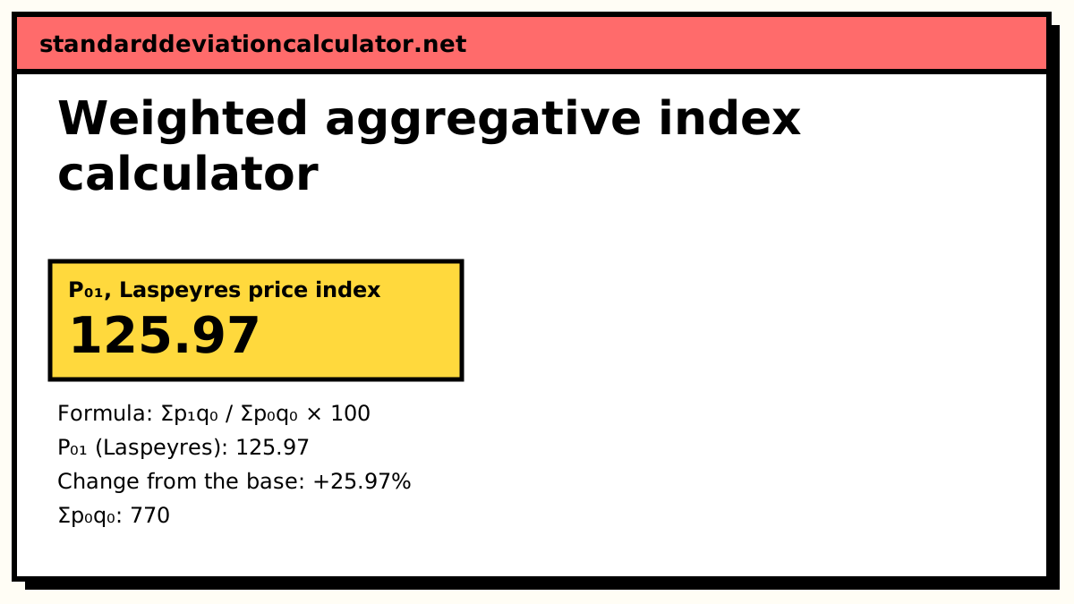
P₀₁ (Laspeyres) = Σp₁q₀ / Σp₀q₀ × 100 = 970 / 770 × 100 = 125.97
P₀₁ = 125.97 means prices in the current period are 25.97% higher than in the base period. Time reversal test: P₁₀ = 81.08, and P₀₁ × P₁₀ = 125.97/100 × 81.08/100 = 1.0214, which is not 1, so the test is not met.
The general formula
P₀₁ = Σp₁w / Σp₀w × 100
Every method in this family prices a basket of quantities w at current prices and at base prices and compares the two totals. The only question is which basket.
| Method | Weight w | Formula | Default data |
|---|---|---|---|
| Laspeyres | q₀ | Σp₁q₀ / Σp₀q₀ × 100 | 125.97 |
| Paasche | q₁ | Σp₁q₁ / Σp₀q₁ × 100 | 123.33 |
| Marshall–Edgeworth | q₀ + q₁ | Σp₁(q₀ + q₁) / Σp₀(q₀ + q₁) × 100 | 124.67 |
| Dorbish–Bowley | — | (L + P) / 2 | 124.65 |
| Fisher | — | √(L × P) | 124.65 |
| Kelly | fixed q | Σp₁q / Σp₀q × 100 | 124.67 |
Dorbish–Bowley and Fisher are averages of Laspeyres and Paasche rather than new baskets. Kelly's row here uses q = (q₀ + q₁)/2, which makes it identical to Marshall–Edgeworth; with a basket from other years, use the Kelly calculator.
A worked example
The default data has five commodities:
| Commodity | p₀ | q₀ | p₁ | q₁ | p₀q₀ | p₁q₀ | p₀q₁ | p₁q₁ |
|---|---|---|---|---|---|---|---|---|
| A | 10 | 20 | 15 | 15 | 200 | 300 | 150 | 225 |
| B | 8 | 15 | 10 | 14 | 120 | 150 | 112 | 140 |
| C | 5 | 30 | 6 | 36 | 150 | 180 | 180 | 216 |
| D | 20 | 10 | 24 | 9 | 200 | 240 | 180 | 216 |
| E | 4 | 25 | 4 | 32 | 100 | 100 | 128 | 128 |
| Σ | 770 | 970 | 750 | 925 |
From the four totals:
- Laspeyres: 970 / 770 × 100 = 125.97 (the calculator's default method).
- Paasche: 925 / 750 × 100 = 123.33.
- Marshall–Edgeworth: (970 + 925) / (770 + 750) × 100 = 1,895 / 1,520 × 100 = 124.67.
- Dorbish–Bowley: (125.97 + 123.33) / 2 = 124.65 (124.654 unrounded).
- Fisher: √(1.25974 × 1.23333) × 100 = 124.65 (124.647 unrounded).
Which methods over- or under-state inflation?
When buyers switch away from goods whose prices rise fastest, as they do in the example (A up 50%, bought less; E unchanged, bought more), the formulas line up in a predictable order:
Paasche ≤ Fisher ≤ Dorbish–Bowley ≤ Laspeyres 123.33 ≤ 124.647 ≤ 124.654 ≤ 125.97
- Laspeyres overstates the rise in the cost of living (upward substitution bias): it prices yesterday's basket, heavy in the goods that became dear.
- Paasche understates it: today's basket has already moved to the goods that became cheap.
- Marshall–Edgeworth, Dorbish–Bowley and Fisher blend the two and land close to the true change. Dorbish–Bowley is never below Fisher, because an arithmetic mean is never below a geometric one.
- Kelly inherits the bias of whatever basket it fixes: an old basket behaves like an old Laspeyres and overstates.
Common questions
What is the weighted aggregative method of index numbers?
Each commodity's price is multiplied by a weight w (a quantity) and the products are
added: P₀₁ = Σp₁w / Σp₀w × 100. The weighted totals are money values, so
commodities quoted in different units can be combined. The methods differ only in the
choice of w.
Which weighted aggregative index is best?
Fisher's ideal index √(L × P) is the one textbooks call best: it lies between Laspeyres and Paasche, uses both years' quantities, and passes both the time reversal and factor reversal tests. Laspeyres is the most used in practice, because it needs only base-year quantities.
Why is Laspeyres higher than Paasche?
Usually because people buy less of what has become dearer. Base-year quantities (Laspeyres) then overweight the items whose prices rose most, and current-year quantities (Paasche) underweight them. In the default data, A rises 50% and its quantity falls from 20 to 15, so L = 125.97 and P = 123.33. If quantities rise where prices rise, the order reverses.
Which methods satisfy the time reversal and factor reversal tests?
Time reversal (P₀₁ × P₁₀ = 1): Marshall–Edgeworth, Fisher and Kelly (fixed weights) pass; Laspeyres, Paasche and Dorbish–Bowley fail. Factor reversal (P₀₁ × Q₀₁ = V₀₁): only Fisher passes. The comparison table under the result checks both on your data.
What is the difference between the simple and weighted aggregative methods?
The simple method adds raw prices, Σp₁ / Σp₀ × 100, so each item counts in
proportion to its price per unit, which depends on the unit it is quoted in. The weighted
method multiplies by quantities first, so each item counts in proportion to what is spent
on it.
Related calculators
-
Laspeyres price index
w = q₀, the base-year basket.
-
Paasche price index
w = q₁, the current-year basket.
-
Fisher’s ideal index
The reversal tests worked in full.
-
Simple aggregative method
The unweighted Σp₁ / Σp₀ × 100.
-
Weighted average of price relatives
The same idea built from relatives, ΣRW / ΣW.