Statistics
Simple aggregative method calculator
The simple aggregative method adds up prices in each year and compares the totals. Enter the base-year and current-year price of each commodity, or switch to quantities for a quantity index.
Add a row for each commodity. Prices must be above zero; quantities and weights cannot be negative.
Add a row for each commodity. Quantities cannot be negative.
Pale bars: p₀ (base year). Solid bars: p₁ (current year). The index compares the total heights, Σp₁ ÷ Σp₀ = 125.53, so the tallest items dominate it.
| Commodity | p₀ | p₁ | p₁ / p₀ × 100 |
|---|---|---|---|
| A | 10 | 15 | 150.00 |
| B | 8 | 10 | 125.00 |
| C | 5 | 6 | 120.00 |
| D | 20 | 24 | 120.00 |
| E | 4 | 4 | 100.00 |
| Σ | 47 | 59 |
Show the working, step by step
Add the base-year prices.
Σp₀ = 10 + 8 + 5 + 20 + 4 = 47
Add the current-year prices.
Σp₁ = 15 + 10 + 6 + 24 + 4 = 59
Divide and multiply by 100.
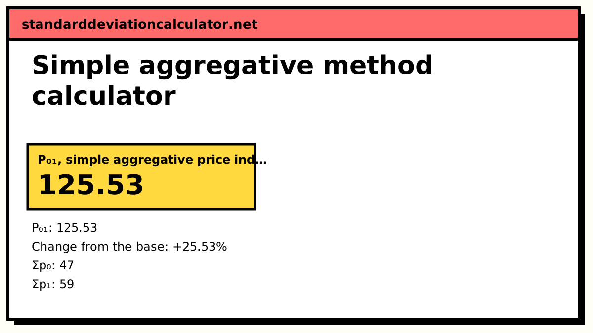
P₀₁ = Σp₁ / Σp₀ × 100 = 59 / 47 × 100 = 125.53
prices in the current period are 25.53% higher than in the base period. D alone is 42.6% of Σp₀, so its change moves the index more than any other item: the method weights each commodity by the size of its price, which depends on the unit it is quoted in.
The formula
P₀₁ = Σp₁ / Σp₀ × 100 Q₀₁ = Σq₁ / Σq₀ × 100
p₀ and p₁ are the prices in the base and current years. The index says how the total price of “one unit of each commodity” has changed. No weights appear, which is why the method is also called the unweighted aggregative method.
A worked example
The calculator's default prices:
| Commodity | p₀ | p₁ |
|---|---|---|
| A | 10 | 15 |
| B | 8 | 10 |
| C | 5 | 6 |
| D | 20 | 24 |
| E | 4 | 4 |
| Σ | 47 | 59 |
- Σp₀ = 10 + 8 + 5 + 20 + 4 = 47.
- Σp₁ = 15 + 10 + 6 + 24 + 4 = 59.
- P₀₁ = 59 / 47 × 100 = 125.53, a rise of 25.53%.
D is the dearest item (20 of the 47), so its 20% rise carries more weight than E's unchanged price, even though nothing tells us people buy more D than E.
The units problem
Suppose E is quoted per 100 units instead of per unit: 400 in both years instead of 4. Nothing about the market has changed, but Σp₀ becomes 443 and Σp₁ becomes 455, and the index falls from 125.53 to 102.71. The item with the biggest price tag dominates the sum, and the size of that price tag is an accident of the unit chosen. This is the main reason the method is taught and then replaced: weighted methods multiply each price by a quantity, turning it into money spent, which does not depend on the unit.
Does it over- or under-state inflation?
There is no fixed direction; it depends on which items happen to have high prices per unit. If expensive items rise faster than cheap ones, the simple aggregative index overstates the general rise; if they rise more slowly, it understates it. Because it ignores quantities, it also has the same blind spot as a Laspeyres index with an equal basket: it cannot see buyers switching to cheaper goods. Here it gives 125.53, higher than the weighted Fisher index of 124.65 for the same prices: E, whose price did not change, is the cheapest item and barely counts in Σp, though buyers spend a good deal on it.
When to use it
- When all items are quoted in the same unit and bought in similar amounts, for example the price of one model of phone across several shops.
- For exam questions that ask for the simple aggregative method by name.
- As a quick first look before collecting quantity data for a weighted index.
Common questions
What is the simple aggregative method of index numbers?
Add the current-year prices of all the commodities, add the base-year prices, and divide:
P₀₁ = Σp₁ / Σp₀ × 100. For the default data, Σp₁ = 59 and Σp₀ = 47, so
P₀₁ = 59 / 47 × 100 = 125.53. It is the simplest index number, and the usual first
method in CBSE Class 12 and B.Com courses.
What are the limitations of the simple aggregative method?
Two main ones. It is affected by the units in which prices are quoted: a commodity priced per quintal dominates one priced per kg. And it gives no weight to how much of each item is actually bought, so a costly item that is rarely purchased can swing the index. Weighted methods such as Laspeyres fix both problems.
How do I calculate a simple aggregative quantity index?
Use quantities in place of prices: Q₀₁ = Σq₁ / Σq₀ × 100. With base
quantities 20, 15, 30, 10, 25 (Σ = 100) and current quantities 15, 14, 36, 9, 32 (Σ = 106),
Q₀₁ = 106.00. Choose “Quantity index” in the calculator. Adding quantities only makes sense
when they are in comparable units.
Does the simple aggregative index satisfy the time reversal test?
Yes. P₁₀ = Σp₀ / Σp₁ × 100, so P₀₁ × P₁₀ = (Σp₁/Σp₀) × (Σp₀/Σp₁) = 1. It does not satisfy the factor reversal test.
What is the difference between the simple aggregative method and the simple average of price relatives?
The aggregative method adds prices first and then divides (Σp₁ / Σp₀), so dear items count for more. The relatives method divides first (p₁ / p₀ for each item) and then averages the percentages, so every item counts equally. On the default data they give 125.53 and 123.00.
Related calculators
-
Simple average of price relatives
Average p₁/p₀ × 100 across items, arithmetic or geometric.
-
Weighted aggregative index
Σp₁w / Σp₀w with quantity weights, six methods.
-
Laspeyres price index
The weighted version most price indices use.
-
Price relatives
p₁/p₀ × 100 per item, plus link and chain relatives.