Skewness calculator
Paste your data to measure how lopsided its distribution is. You get the skewness figures that Excel, SPSS, Minitab and textbooks use, a test of whether the skew is real, and a histogram.
Separate with commas, spaces or new lines. At least 3 values.
Show the working, step by step
Find the mean and the second and third central moments (dividing by n).
x̄ = 5.33333 m₂ = Σ(x − x̄)² ÷ n = 88.6667 ÷ 12 = 7.38889 m₃ = Σ(x − x̄)³ ÷ n = 280.889 ÷ 12 = 23.4074
Fisher–Pearson coefficient.
g₁ = m₃ ÷ m₂3/2 = 23.4074 ÷ 20.0849 = 1.165
Adjust for sample size (the figure Excel’s SKEW reports).
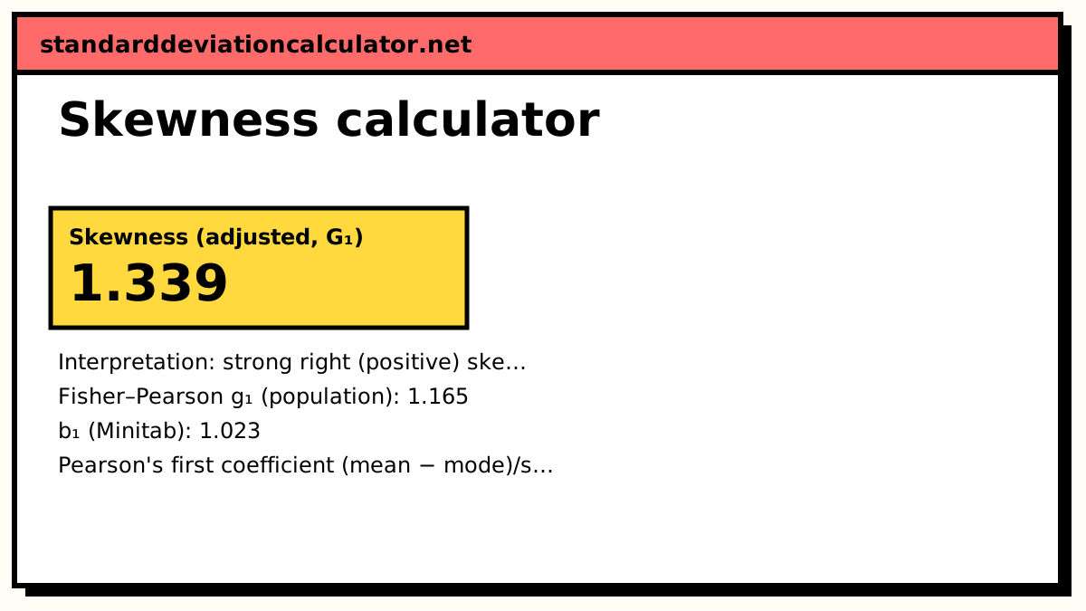
G₁ = g₁ × √(n(n − 1)) ÷ (n − 2) = 1.165 × √(12 × 11) ÷ 10 = 1.339
Pearson's coefficients use the sample SD.
s = 2.83912 second: 3 × (5.33333 − 4.5) ÷ 2.83912 = 0.8806 first: (5.33333 − 4) ÷ 2.83912 = 0.4696
Test whether the skew could be chance.
SES = √(6n(n − 1) ÷ ((n − 2)(n + 1)(n + 3))) = 0.6373 z = 1.339 ÷ 0.6373 = 2.101, p = 0.03564
|z| > 1.96, so the skew is significant at the 5% level: the population is probably not symmetric.
The formulas
m₂ = Σ(x − x̄)² ÷ n m₃ = Σ(x − x̄)³ ÷ n g₁ = m₃ ÷ m₂3/2 G₁ = g₁ × √(n(n − 1)) ÷ (n − 2) Pearson 1 = (x̄ − mode) ÷ s Pearson 2 = 3(x̄ − median) ÷ s SES = √(6n(n − 1) ÷ ((n − 2)(n + 1)(n + 3)))
Cubing the deviations keeps their signs, so large deviations above the mean push m₃ up and large deviations below push it down. Dividing by m₂3/2 makes the result unit-free.
A worked example
The default data are 12 values: 2, 3, 3, 4, 4, 4, 5, 5, 6, 7, 9, 12.
- The mean is 64 ÷ 12 = 5.333. The squared deviations add to 88.67 and the cubed deviations to 280.9, so m₂ = 88.67 ÷ 12 = 7.389 and m₃ = 280.9 ÷ 12 = 23.41.
- g₁ = 23.41 ÷ 7.3891.5 = 23.41 ÷ 20.08 = 1.165.
- G₁ = 1.165 × √(12 × 11) ÷ 10 = 1.339. This is the number Excel's SKEW returns.
- With s = 2.839, median 4.5 and mode 4: Pearson's second coefficient is 3 × (5.333 − 4.5) ÷ 2.839 = 0.881, and the first is (5.333 − 4) ÷ 2.839 = 0.470.
- SES for n = 12 is 0.637, so z = 1.339 ÷ 0.637 = 2.10 with a two-sided p-value of 0.036.
Interpreting the result
G₁ = 1.34 is above 1, so by the usual rule of thumb the sample is highly right-skewed: most values bunch between 2 and 7 and a few (9, 12) stretch the right tail. The mean (5.33) sits above the median (4.5), which sits above the mode (4), the classic order for right skew.
The z test says the skew is significant at the 5% level (|z| = 2.10 > 1.96), so a symmetric population would rarely produce a sample this lopsided. With only 12 values, though, the estimate is rough: change the 12 to 8 and G₁ drops to 0.61. Skewness is sensitive to the most extreme values, so check them before drawing conclusions.
For analysis, strong right skew suggests reporting the median rather than the mean, or taking logs before a t-test. Mild skew (under about 0.5) rarely matters for tests on the mean with moderate samples.
Common mistakes
- Comparing a G₁ from Excel with a g₁ from a textbook and concluding one is wrong. Check which formula each uses.
- Reading the sign backwards. Right skew is positive and means a long tail of large values, not that the bulk of the data is on the right.
- Trusting skewness from very small samples. Below about 20 values the standard error is large.
- Using Pearson's first coefficient when the data have no single mode.
Common questions
What does skewness tell you?
Which way, and how strongly, a distribution leans. Positive (right) skew means a long tail of large values, as with incomes or house prices; the mean is then usually above the median. Negative (left) skew means a long tail of small values, as with scores on an easy test. Zero means the two tails balance.
Why do different programs give different skewness values?
They use different formulas. Excel's SKEW, SPSS and SAS report the adjusted G₁; R's
e1071::skewness defaults to b₁ (the Minitab version); many textbooks and SciPy's
default give the population g₁. All three agree for large samples. For the default data they
are 1.339, 1.023 and 1.165.
What skewness value counts as highly skewed?
A common rule of thumb (Bulmer, 1979): between −0.5 and 0.5 is approximately symmetric, 0.5 to 1 in either direction is moderately skewed, and beyond ±1 is highly skewed. For small samples also look at the standard error: a skewness of 1 from 10 values is not strong evidence of anything.
How do I test whether skewness is significant?
Divide G₁ by its standard error, SES = √(6n(n − 1) ÷ ((n − 2)(n + 1)(n + 3))). If |z| is greater than 1.96, the skew is significant at the 5% level. This is the test SPSS users apply by hand to the skewness and its standard error in the Descriptives output.
What are Pearson's coefficients of skewness?
Older, simpler measures. The first is (mean − mode) ÷ s; the second is 3(mean − median) ÷ s. They use the fact that the mean is pulled toward the long tail more than the median or mode. The second is more stable, because a sample's mode can jump around or not exist.
Related calculators
-
Descriptive statistics calculator
Mean, SD, quartiles, skewness and kurtosis together.
-
Histogram maker
See the shape of the distribution the skewness describes.
-
Outlier calculator
Check whether one extreme value is causing the skew.