Exponential growth prediction calculator
Project a quantity that grows by a fixed percentage each period. Enter any three of the start value, rate, time and end value, and the calculator solves for the fourth and draws the curve.
Negative for decay, e.g. −3.
Ignored when solving for x(t).
| t | x(t) |
|---|---|
| 0 | 1000 |
| 1 | 1050 |
| 2 | 1102.5 |
| 3 | 1157.63 |
| 4 | 1215.51 |
| 5 | 1276.28 |
| 6 | 1340.1 |
| 7 | 1407.1 |
| 8 | 1477.46 |
| 9 | 1551.33 |
| 10 | 1628.89 |
Show the working, step by step
The model:
x(t) = x₀ · (1 + r)^t
Rate as a decimal:
r = 5% = 0.05
Rearrange for the unknown and substitute.
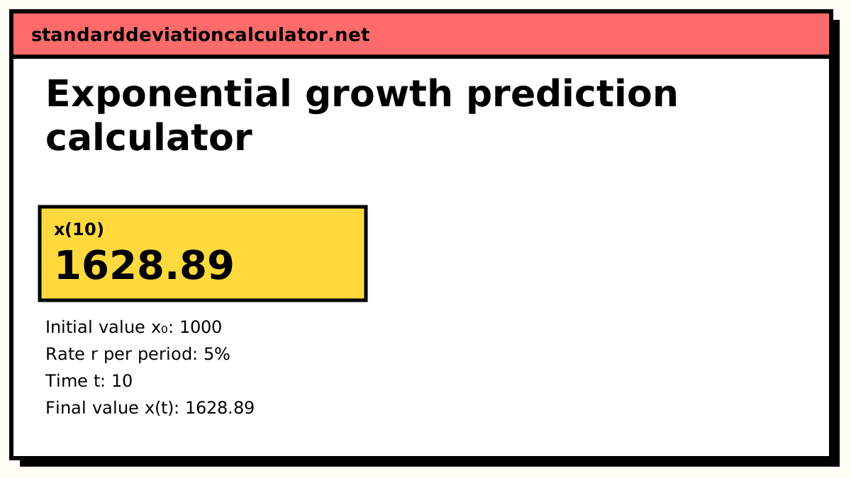
x(10) = 1000 × (1 + 0.05)^10 = 1000 × 1.62889 = 1628.89
Doubling time:
ln 2 ÷ |ln(1 + r)| = 0.693147 ÷ 0.0487902 = 14.2067
A prediction from this model assumes the rate stays constant for the whole period. Real growth usually slows as it meets limits.
The formula
x(t) = x₀ · (1 + r)^t (discrete) x(t) = x₀ · e^(r·t) (continuous)
Here x₀ is the value at time 0, r is the growth rate per period written as a decimal (5% is 0.05), and t is the number of periods. The discrete form fits anything that changes once per period by a set percentage, such as annual interest or a yearly price rise. The continuous form fits processes that compound all the time, such as bacterial growth or radioactive decay described by a rate constant.
Each form can be rearranged for any of its parts:
x₀ = x(t) ÷ (1 + r)^t r = (x(t) ÷ x₀)^(1/t) − 1 t = ln(x(t) ÷ x₀) ÷ ln(1 + r)
A worked example
The default inputs start at x₀ = 1,000 and grow 5% per period for 10 periods, using the discrete model.
x(10) = 1000 × 1.05^10 = 1000 × 1.62889 = 1628.89
The quantity grows by a factor of 1.62889, so it ends about 63% higher, not 50% higher as simple (non-compounding) growth would give. The extra 13 percentage points come from growth on growth: each period's 5% applies to a larger base than the last.
The doubling time is ln 2 ÷ ln 1.05 = 0.693147 ÷ 0.0487902 = 14.207 periods. The equivalent continuous rate is ln 1.05 = 4.879%, which means 5% compounded once per period matches 4.879% compounded continuously.
Switch the model to continuous and the same inputs give 1000 × e0.5 = 1648.72, slightly more because the growth compounds without pause. Switch "Solve for" to growth rate, keep x(t) = 2,000, and the rate needed to double in 10 periods is 7.1773% per period.
How to read the prediction
An exponential prediction is only as good as the assumption that the rate stays fixed. Over a few periods that is often reasonable. Over long spans it rarely holds: populations run out of food or space, sales saturate a market, and an early 40% growth rate cannot continue for decades. If your data bends away from a straight line on a log scale, a logistic or other limited-growth model is a better fit.
The period is whatever unit you choose: years, months, hours or generations. The rate and the time must use the same unit. A 12% annual rate is not a 12% monthly rate; the matching monthly rate is 1.121/12 − 1 = 0.949%.
To estimate a rate from past data, take the first and last values and the number of periods between them. That gives the compound average growth rate, which smooths over ups and downs in between. It does not tell you how variable the growth was.
Common mistakes
- Entering the rate as 0.05 when the field expects a percentage. The calculator takes 5 for 5%.
- Mixing units, such as an annual rate with a time in months.
- Using the continuous formula with a percentage quoted as an annual effective rate. They differ: 5% effective is 4.879% continuous.
- Adding the rate each period (1000 + 10 × 50) instead of compounding it. That is linear growth.
- Trusting a long-range forecast from a short run of data. Small errors in r grow exponentially too.
Common questions
What is the exponential growth formula?
For growth by a fixed percentage each period, x(t) = x₀(1 + r)t, where x₀ is the starting value, r the rate per period as a decimal and t the number of periods. For growth that compounds continuously, x(t) = x₀ert. With x₀ = 1,000, r = 5% and t = 10, the first gives 1,628.89 and the second 1,648.72.
How do I find the growth rate from two values?
Rearrange the formula: r = (x(t) ÷ x₀)1/t − 1. Going from 1,000 to 2,000 in 10 periods gives r = 20.1 − 1 = 0.071773, or 7.1773% per period. For the continuous model, r = ln(x(t) ÷ x₀) ÷ t = 6.9315%.
How long does it take to double?
The doubling time is ln 2 ÷ ln(1 + r) periods, or ln 2 ÷ r for continuous growth. At 5% per period that is 14.21 periods (13.86 if continuous). The rule of 70 (70 ÷ 5 = 14) is a quick mental version that works well for small rates.
Does the calculator handle decay?
Yes. Enter a negative rate, such as −3, and the curve falls instead of rising. The doubling time becomes a half-life: the number of periods for the quantity to halve, which is ln 2 ÷ |ln(1 − 0.03)| ≈ 22.76 periods.
Can I use a fractional or negative time?
Yes. Time can be any real number. A fractional t gives the value partway through a period under smooth compounding, and a negative t runs the model backwards to estimate an earlier value.
Related calculators
-
Compound interest calculator
The same growth formula applied to money, with deposits and compounding frequency.
-
Inflation calculator
Price growth over time at a fixed annual rate.
-
Graphing calculator
Plot any exponential or logarithmic function.