Effect size calculator
Measure how big an effect is, not just whether it is significant. Enter two group means, SDs and sizes, or a t, r, d or F value you already have, and the calculator gives the standard effect sizes and converts between them.
┄ Group 2 (control) ━ Group 1 (treatment)
The curves overlap by 71.2%; a random member of group 1 beats one from group 2 69.9% of the time.
| Measure | Standardiser | Value |
|---|---|---|
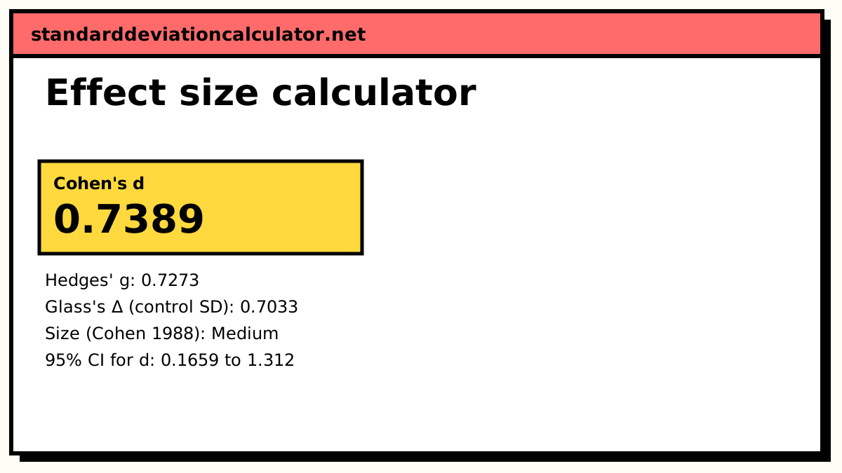
| Cohen's d | Pooled SD sp | 0.7389 |
| Hedges' g | Pooled SD, bias-corrected | 0.7273 |
| Glass's Δ | Control group SD s₂ | 0.7033 |
| r (point-biserial) | – | 0.3465 |
Show the working, step by step
Pool the two standard deviations.
sp = √(((n₁ − 1)s₁² + (n₂ − 1)s₂²) ÷ (n₁ + n₂ − 2)) = √((24 × 8.2² + 24 × 9.1²) ÷ 48) = 8.6617
Cohen's d is the mean difference in pooled-SD units.
d = (78.5 − 72.1) ÷ 8.6617 = 6.4 ÷ 8.6617 = 0.738885
Hedges' g removes the small-sample bias in d.
J = 1 − 3 ÷ (4 × 48 − 1) = 0.984293 g = 0.738885 × 0.984293 = 0.72728
Glass's Δ uses only the control group's SD, useful when the treatment changes the spread.
Δ = 6.4 ÷ 9.1 = 0.703297
Convert d to a correlation.
a = (n₁ + n₂)² ÷ (n₁n₂) = 4 r = d ÷ √(d² + a) = 0.346549
The confidence interval uses the large-sample standard error √((n₁ + n₂)/(n₁n₂) + d²/(2(n₁ + n₂))).
The formulas
sp = √(((n₁ − 1)s₁² + (n₂ − 1)s₂²) ÷ (n₁ + n₂ − 2)) Cohen's d = (x̄₁ − x̄₂) ÷ sp Hedges' g = d × (1 − 3 ÷ (4(n₁ + n₂ − 2) − 1)) Glass's Δ = (x̄₁ − x̄₂) ÷ s₂ d = t × √(1/n₁ + 1/n₂) r = d ÷ √(d² + 4), d = 2r ÷ √(1 − r²) η² = F·df₁ ÷ (F·df₁ + df₂), f = √(η² ÷ (1 − η²))
A worked example
The default compares a treatment group (mean 78.5, SD 8.2, n = 25) with a control group (mean 72.1, SD 9.1, n = 25). First pool the SDs:
sp = √((24 × 8.2² + 24 × 9.1²) ÷ 48) = 8.6617 d = (78.5 − 72.1) ÷ 8.6617 = 6.4 ÷ 8.6617 = 0.7389
Hedges' correction factor with 48 degrees of freedom is 1 − 3 ÷ 191 = 0.984293, so g = 0.7273. Glass's Δ divides by the control SD only: 6.4 ÷ 9.1 = 0.7033. The equivalent correlation is r = 0.7389 ÷ √(0.7389² + 4) = 0.3465.
By Cohen's benchmarks d = 0.74 is a medium effect, close to large. The 95% confidence interval runs from 0.166 to 1.312, which is wide: with 25 per group the data are consistent with anything from a small to a very large effect.
The other inputs
If a paper gives only t = 2.61 with 25 per group, the t mode returns d = 2.61 × √(1/25 + 1/25) = 0.7382, almost the same as above. From a correlation r = 0.3 the r mode gives d = 0.629. From d = 0.5 the d mode gives r = 0.2425. For an ANOVA with F = 4.2 on 2 and 57 degrees of freedom, η² = 8.4 ÷ 65.4 = 0.1284, so the factor explains about 12.8% of the variance, and Cohen's f = 0.3839.
How to interpret d
d measures the gap between two means in standard deviations. The calculator also turns it into statements about overlap, assuming normal data with equal spread. For d = 0.7389:
- U₃ = 77%: the average treated person scores above 77% of the control group.
- The two distributions overlap by 71.2%.
- The probability of superiority is 69.9%: pick one person from each group at random, and the treated one scores higher about 70% of the time.
These are often easier to explain to a non-statistical audience than a bare 0.74. Whether the effect is important depends on context: a d of 0.2 on mortality is large in practical terms, while a d of 0.8 on a lab reaction-time task may be routine.
Choosing the right measure
Use d or g for two group means, r for two continuous variables, and η² (or f) for ANOVA factors. Convert only when you need to combine studies on one scale, and say which conversion you used, because the r ↔ d formulas assume equal groups unless you supply the sizes.
Common mistakes
- Using the formula d = t × √(1/n₁ + 1/n₂) on a paired t-test. For paired data use dz = t ÷ √n, and say so.
- Swapping the groups in Glass's Δ. The denominator should be the control or baseline group's SD.
- Reading "medium" as a verdict. Cohen's labels are rough defaults, not measures of importance.
- Comparing partial η² from a multi-factor design with η² from a one-way ANOVA.
- Dropping the sign. A negative d just means group 2 had the higher mean; report the direction in words.
Common questions
What is an effect size?
A number that says how large a difference or relationship is, on a scale that does not depend on the sample size. A p-value tells you whether an effect is distinguishable from zero; an effect size tells you how big it is. Cohen's d, Hedges' g, r and η² are all effect sizes, measured in different units.
Which should I report: Cohen's d, Hedges' g or Glass's Δ?
Report d or g when the two groups have similar spreads. g is d with a small-sample correction and is the usual choice in meta-analysis. Use Glass's Δ when the treatment is likely to change the spread as well as the mean, because it standardises by the control group's SD alone. For more on d itself, see the Cohen's d calculator.
How do I convert between r and d?
For two groups of equal size, d = 2r ÷ √(1 − r²) and r = d ÷ √(d² + 4). With unequal groups, replace 4 with (n₁ + n₂)² ÷ (n₁n₂). So r = 0.3 corresponds to d = 0.629, and d = 0.5 to r = 0.243.
What are small, medium and large effects?
Cohen's benchmarks are 0.2, 0.5 and 0.8 for d; 0.1, 0.3 and 0.5 for r; and 0.01, 0.06 and 0.14 for η². Cohen himself called them a last resort for when a field has no better reference. The labels for d and r do not line up exactly: r = 0.3 is "medium" but converts to d = 0.63.
Is η² from F the same as partial η²?
The formula η² = F·df₁ ÷ (F·df₁ + df₂) gives partial η² for the effect whose F you enter. In a one-way ANOVA there is only one effect, so partial η² and η² are the same number. In designs with several factors, partial η² values can add up to more than 1 and should not be compared across designs.
Related calculators
-
Cohen's d calculator
Cohen's d from two group means and SDs, with its confidence interval.
-
T-test calculator
Test whether two means differ, then size the difference here.
-
ANOVA calculator
One-way ANOVA with the F statistic to turn into η².