T table (Student's t critical values)
A t table lists the critical values of Student's t distribution: the cut-offs beyond which a test result is significant. Use the lookup box for any df, any α or an observed t, or read the printed two-tailed table below, from df 1 to ∞.
0.05 is the usual choice.
n − 1 for a one-sample test, n₁ + n₂ − 2 for a pooled two-sample test.
The t statistic your test produced, positive or negative.
Show the working, step by step
A two-tailed test splits α between the two tails, so each tail holds α/2 and the cut-off has 1 − α/2 of the distribution below it.
Read it from the t table (row df = 18, column α = 0.05) or compute it:
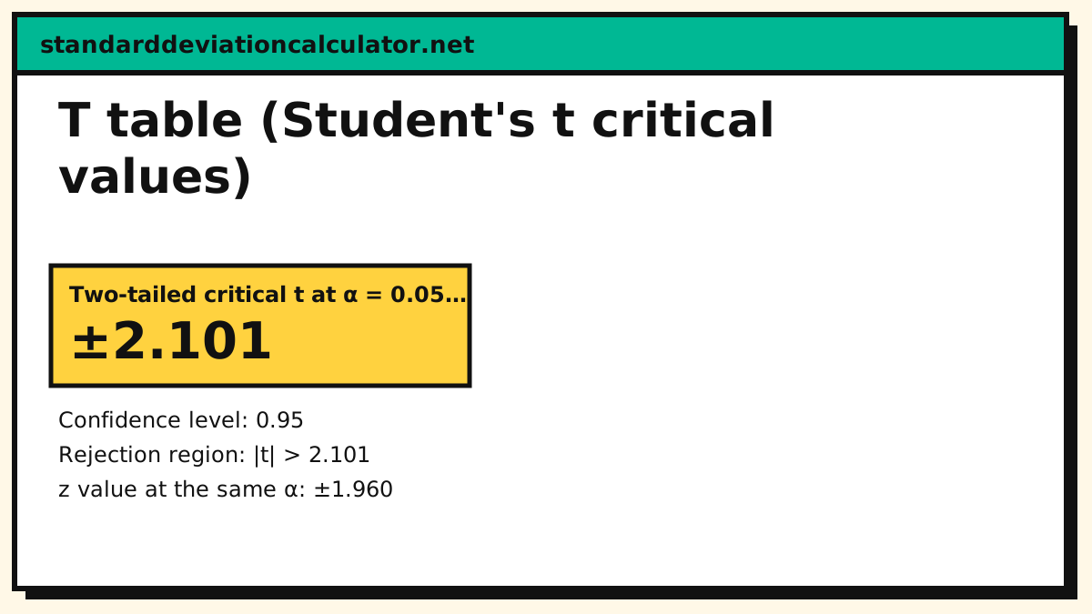
t* = ±2.101
The t value is always a little further out than the z value, because estimating the standard deviation costs precision. As df grows the two converge:
t* 2.101 against z* 1.960
The printed two-tailed table below lists the usual α levels; this tool handles any α and one-tailed lookups.
How to read a t table
The rows are the degrees of freedom and the columns are the significance levels. The table below is two-tailed: the number in a cell is the value t* such that α of the t distribution's area sits in both tails combined.
Worked lookup for df = 18, α = 0.05, two-tailed:
- Find the row df = 18.
- Find the column 0.05.
- The cell reads 2.101 (highlighted below).
- A two-tailed test rejects H₀ when |t| > 2.101; a confidence interval multiplies the standard error by 2.101.
The one-tailed value at α = 0.05 is the 0.10 column of this table (1.734 at df = 18), because a one-tailed test puts all of α in one end instead of splitting it.
| df | 0.1 | 0.05 | 0.02 | 0.01 | 0.005 |
|---|---|---|---|---|---|
| 1 | 6.314 | 12.706 | 31.821 | 63.657 | 127.321 |
| 2 | 2.920 | 4.303 | 6.965 | 9.925 | 14.089 |
| 3 | 2.353 | 3.182 | 4.541 | 5.841 | 7.453 |
| 4 | 2.132 | 2.776 | 3.747 | 4.604 | 5.598 |
| 5 | 2.015 | 2.571 | 3.365 | 4.032 | 4.773 |
| 6 | 1.943 | 2.447 | 3.143 | 3.707 | 4.317 |
| 7 | 1.895 | 2.365 | 2.998 | 3.499 | 4.029 |
| 8 | 1.860 | 2.306 | 2.896 | 3.355 | 3.833 |
| 9 | 1.833 | 2.262 | 2.821 | 3.250 | 3.690 |
| 10 | 1.812 | 2.228 | 2.764 | 3.169 | 3.581 |
| 15 | 1.753 | 2.131 | 2.602 | 2.947 | 3.286 |
| 18 | 1.734 | 2.101 | 2.552 | 2.878 | 3.197 |
| 20 | 1.725 | 2.086 | 2.528 | 2.845 | 3.153 |
| 25 | 1.708 | 2.060 | 2.485 | 2.787 | 3.078 |
| 30 | 1.697 | 2.042 | 2.457 | 2.750 | 3.030 |
| 40 | 1.684 | 2.021 | 2.423 | 2.704 | 2.971 |
| 50 | 1.676 | 2.009 | 2.403 | 2.678 | 2.937 |
| 60 | 1.671 | 2.000 | 2.390 | 2.660 | 2.915 |
| 100 | 1.660 | 1.984 | 2.364 | 2.626 | 2.871 |
| ∞ | 1.645 | 1.960 | 2.326 | 2.576 | 2.807 |
One-tailed values from the two-tailed table
Printed two-tailed tables double up as one-tailed ones: the one-tailed α is the two-tailed 2α. The most-used pairs, at df = 18:
| One-tailed α | Two-tailed α | Critical t, df 18 | Typical use |
|---|---|---|---|
| 0.10 | 0.20 | 1.330 | Directional test at 10% |
| 0.05 | 0.10 | 1.734 | Directional test at 5% |
| 0.025 | 0.05 | 2.101 | Two-tailed test at 5%, or 95% CI |
| 0.01 | 0.02 | 2.552 | Two-tailed test at 2%, or 98% CI |
A worked significance test
A sample of n = 19 readings gives t = 2.4 against H₀: μ = 100. The df are n − 1 = 18, so the two-tailed 5% cut-off is 2.101 from the table above. Because 2.4 > 2.101, the result is significant at the 5% level. The lookup box above gives the exact p-value for t = 2.4 at df = 18; the t-test calculator runs the whole test from raw data.
Why the t table is not just the z table
When the standard deviation is estimated from the sample instead of known, the test statistic carries that extra uncertainty and its distribution has heavier tails: a 2.0 is a normal two-sided 0.046 event but a 0.061 event at df = 18. Every row of the t table is therefore further from zero than the ∞ (z) row, and the gap closes as the sample grows — df 100 needs only 1.984 where z needs 1.960. That is why the t table exists at all: the normal table is wrong by exactly this amount for small samples, and that amount is not small when n is 5.
The values are computed by the same inverse-CDF routine as the critical value calculator, not transcribed from a printed table, and rounded to 3 decimal places — the standard for t.
Common questions
How do you read a t table?
Find your degrees of freedom down the left column and your significance level across the top. The cell where they meet is the critical value t*. For a two-tailed test at α = 0.05 with df = 18 that cell reads 2.101: reject the null when |t| exceeds 2.101. Most printed t tables are two-tailed; the lookup box above handles either convention.
How do I find the degrees of freedom?
They come from the test, not the table. A one-sample or paired t-test has df = n − 1; a pooled two-sample t-test has df = n₁ + n₂ − 2. A confidence interval for a mean uses the same df as the test would. The degrees of freedom calculator works it out from your sample sizes.
What is the critical t value at 95% with 18 degrees of freedom?
±2.101 for a two-tailed test. That is the row df = 18, column 0.05 cell of the table above. It is the multiplier in a 95% confidence interval for a mean with n = 19, and the cut-off for a two-tailed test at the 5% level. Compare z: with known σ the same interval would use 1.960; the extra 0.141 is the price of estimating σ.
How is a one-tailed t table different?
The same numbers, read with the α doubled. A one-tailed test at α = 0.05 has the same cut-off as a two-tailed test at α = 0.10, so it is the 0.10 column, not the 0.05 column: with df = 18 that is 1.734 against 2.101. One-tailed tests are easier to pass, which is why the direction must be fixed before the data are seen.
Why does the t table have a row for infinite df?
The ∞ row is the normal (z) limit: as the sample grows, estimating σ costs less, the t distribution becomes the normal distribution, and the 0.05 two-tailed value settles at 1.960. That is the last row of the table above and why textbooks note "use z when n is large". For df = 100 the value is 1.984, already close.
Related calculators
-
T-test calculator
Run the test that gives you the t statistic to look up.
-
Critical value calculator
z, t, chi-square and F critical values at any α.
-
Confidence interval
The two-tailed critical value is its multiplier.
-
Chi-square table
The upper-tail counterpart for tests on counts.
-
F table
Critical F values for ANOVA and two-variance tests.