F table (critical values)
An F table lists the critical values of the F distribution, which needs two degrees of freedom because it is a ratio of two variance estimates. Use the lookup box for any df₁, df₂, α or an observed F, or read the printed 0.05 and 0.01 tables below, from df 1 to ∞.
0.05 is the usual choice.
Groups − 1 in one-way ANOVA; the first variance estimate’s df.
Total observations − groups in one-way ANOVA; the second variance estimate’s df.
The F statistic your test produced.
Show the working, step by step
The critical value is the point with α = 0.05 of the F distribution's area in the upper tail, at the two given degrees of freedom.
Read it from the table (column df₁, row df₂) or compute it:
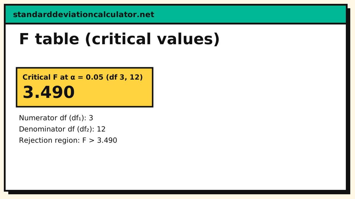
F* = 3.490
F tables are not symmetric in their df, so read across with the numerator df and down with the denominator df — swapping them is a different table.
F* for df (12, 3) instead is 8.745
The printed table below covers α = 0.05 with the usual df combinations; this tool handles any α and any df.
How to read an F table
The columns are the numerator degrees of freedom df₁ and the rows the denominator df₂. A cell is the value with α of the F distribution's area in the upper tail. The test is always upper-tailed: large F, the two variances differ enough.
Worked lookup for df₁ = 3, df₂ = 10, α = 0.05:
- Find the column df₁ = 3.
- Find the row df₂ = 10.
- The cell reads 3.708 (highlighted below).
- Reject H₀ when the computed F exceeds 3.708.
In a one-way ANOVA, df₁ is the number of groups minus one and df₂ is the total observations minus the number of groups, so most lookups land on small df₁ against a larger df₂.
| df₂ | 1 | 2 | 3 | 4 | 5 | 10 | 20 | 30 | 60 | 120 | ∞ |
|---|---|---|---|---|---|---|---|---|---|---|---|
| 1 | 161.448 | 199.500 | 215.707 | 224.583 | 230.162 | 241.882 | 248.013 | 250.095 | 252.196 | 253.253 | 254.314 |
| 2 | 18.513 | 19.000 | 19.164 | 19.247 | 19.296 | 19.396 | 19.446 | 19.462 | 19.479 | 19.487 | 19.496 |
| 3 | 10.128 | 9.552 | 9.277 | 9.117 | 9.013 | 8.786 | 8.660 | 8.617 | 8.572 | 8.549 | 8.526 |
| 4 | 7.709 | 6.944 | 6.591 | 6.388 | 6.256 | 5.964 | 5.803 | 5.746 | 5.688 | 5.658 | 5.628 |
| 5 | 6.608 | 5.786 | 5.409 | 5.192 | 5.050 | 4.735 | 4.558 | 4.496 | 4.431 | 4.398 | 4.365 |
| 10 | 4.965 | 4.103 | 3.708 | 3.478 | 3.326 | 2.978 | 2.774 | 2.700 | 2.621 | 2.580 | 2.538 |
| 15 | 4.543 | 3.682 | 3.287 | 3.056 | 2.901 | 2.544 | 2.328 | 2.247 | 2.160 | 2.114 | 2.066 |
| 20 | 4.351 | 3.493 | 3.098 | 2.866 | 2.711 | 2.348 | 2.124 | 2.039 | 1.946 | 1.896 | 1.843 |
| 30 | 4.171 | 3.316 | 2.922 | 2.690 | 2.534 | 2.165 | 1.932 | 1.841 | 1.740 | 1.683 | 1.622 |
| 40 | 4.085 | 3.232 | 2.839 | 2.606 | 2.449 | 2.077 | 1.839 | 1.744 | 1.637 | 1.577 | 1.509 |
| 60 | 4.001 | 3.150 | 2.758 | 2.525 | 2.368 | 1.993 | 1.748 | 1.649 | 1.534 | 1.467 | 1.389 |
| 120 | 3.920 | 3.072 | 2.680 | 2.447 | 2.290 | 1.910 | 1.659 | 1.554 | 1.429 | 1.352 | 1.254 |
| ∞ | 3.841 | 2.996 | 2.605 | 2.372 | 2.214 | 1.831 | 1.571 | 1.459 | 1.318 | 1.221 | NaN |
| df₂ | 1 | 2 | 3 | 4 | 5 | 10 | 20 | 30 | 60 | 120 | ∞ |
|---|---|---|---|---|---|---|---|---|---|---|---|
| 1 | 4052.181 | 4999.500 | 5403.352 | 5624.583 | 5763.650 | 6055.847 | 6208.730 | 6260.649 | 6313.030 | 6339.391 | 6365.864 |
| 2 | 98.503 | 99.000 | 99.166 | 99.249 | 99.299 | 99.399 | 99.449 | 99.466 | 99.482 | 99.491 | 99.499 |
| 3 | 34.116 | 30.817 | 29.457 | 28.710 | 28.237 | 27.229 | 26.690 | 26.505 | 26.316 | 26.221 | 26.125 |
| 4 | 21.198 | 18.000 | 16.694 | 15.977 | 15.522 | 14.546 | 14.020 | 13.838 | 13.652 | 13.558 | 13.463 |
| 5 | 16.258 | 13.274 | 12.060 | 11.392 | 10.967 | 10.051 | 9.553 | 9.379 | 9.202 | 9.112 | 9.020 |
| 10 | 10.044 | 7.559 | 6.552 | 5.994 | 5.636 | 4.849 | 4.405 | 4.247 | 4.082 | 3.996 | 3.909 |
| 15 | 8.683 | 6.359 | 5.417 | 4.893 | 4.556 | 3.805 | 3.372 | 3.214 | 3.047 | 2.959 | 2.868 |
| 20 | 8.096 | 5.849 | 4.938 | 4.431 | 4.103 | 3.368 | 2.938 | 2.778 | 2.608 | 2.517 | 2.421 |
| 30 | 7.562 | 5.390 | 4.510 | 4.018 | 3.699 | 2.979 | 2.549 | 2.386 | 2.208 | 2.111 | 2.006 |
| 40 | 7.314 | 5.179 | 4.313 | 3.828 | 3.514 | 2.801 | 2.369 | 2.203 | 2.019 | 1.917 | 1.805 |
| 60 | 7.077 | 4.977 | 4.126 | 3.649 | 3.339 | 2.632 | 2.198 | 2.028 | 1.836 | 1.726 | 1.601 |
| 120 | 6.851 | 4.787 | 3.949 | 3.480 | 3.174 | 2.472 | 2.035 | 1.860 | 1.656 | 1.533 | 1.381 |
| ∞ | 6.635 | 4.605 | 3.782 | 3.319 | 3.017 | 2.321 | 1.878 | 1.696 | 1.473 | 1.325 | NaN |
Where the F distribution comes from
An F statistic is the ratio of two independent mean squares, each an unbiased estimate of the same variance. Under the null it is a ratio of two chi-square variables divided by their degrees of freedom, which is the F distribution. Two tests use the table directly:
- One-way ANOVA over k groups uses df₁ = k − 1 and df₂ = N − k, and the ANOVA calculator returns the F you compare against this table.
- Comparing two variances uses the ratio of the two sample variances with df₁ = n₁ − 1 and df₂ = n₂ − 1, which the F-test calculator sets up. The ratio convention is larger-over-smaller when you only want "do they differ", but keep the direction when the test is one-sided.
The reciprocal property
If X follows F(df₁, df₂), then 1/X follows F(df₂, df₁), so the upper-tail cut-off of one direction equals the reciprocal of the upper-tail cut-off of the swapped direction at the complementary probability: F(α; df₁, df₂) = 1 ÷ F(1 − α; df₂, df₁). For example F(0.05; 3, 10) = 3.708 = 1 ÷ F(0.95; 10, 3) = 1 ÷ 0.270. That is why printing only the upper tail is complete: the lower-tail cut-off you need at (df₁, df₂) is the reciprocal of the swapped table value at 1 − α, and the lookup box works the reciprocal out for you.
The values are computed by the same inverse-CDF routine as the critical value calculator, not transcribed from a printed table, and rounded to 3 decimal places. The ∞ row and column use the χ² limiting identities, which agree with the finite-df inverse CDF to two decimal places by df 3,000 (the printed table rounds to three, and the last third of a printed unit is a slow convergence, not a mismatch).
Common questions
How do you read an F table?
An F table needs two numbers: the numerator degrees of freedom df₁ (across the top) and the denominator degrees of freedom df₂ (down the side). The cell where the df₁ column and the df₂ row meet is the critical value. For df₁ = 3, df₂ = 10 at α = 0.05 that cell is 3.708: reject the null when the F statistic exceeds it. Because the F statistic is a ratio of variances, it is always positive and the test is upper-tailed.
How do I find df₁ and df₂ for an ANOVA F test?
For one-way ANOVA over k groups from N total observations, df₁ = k − 1 (numerator, the between-groups df) and df₂ = N − k (denominator, the within-groups df). Three groups of ten gives df₁ = 2, df₂ = 27. The degrees of freedom calculator works out both from your group sizes.
What is the critical F value for df₁ = 3, df₂ = 12 at α = 0.05?
3.490 — the column df₁ = 3, row df₂ = 12 cell of the 0.05 table above. The critical value calculator returns the same figure and handles any df combination not in the printed table.
Why is the F table not symmetric when I swap df₁ and df₂?
Because F is a ratio of two variance estimates, the table is a grid, not a triangle: the cell at df₁ = 3, df₂ = 10 (3.708) and the cell at df₁ = 10, df₂ = 3 (8.786) are different numbers at the same α. What does hold is the complementary reciprocal: the upper-tail value F(0.05; 3, 10) = 3.708 equals 1 ÷ F(0.95; 10, 3) = 1 ÷ 0.270. Read across with the numerator df and down with the denominator df; a lower-tail cut-off at one direction is the reciprocal of an upper-tail cut-off in the other direction at the complementary α.
What do the ∞ row and ∞ column mean?
They are the limits of the F distribution. Along the bottom ∞ row (df₂ → ∞) the denominator estimate χ²(df₂)/df₂ converges to 1, so the critical value reduces to χ²(df₁)/df₁ — the chi-square cut-off divided by its df. Along the right ∞ column (df₁ → ∞) the numerator converges to 1, and the value is df₂/χ²(df₂; 0.95). That is why a one-way ANOVA against a known variance is a chi-square test in disguise: its F table row collapses to χ²(df)/df.
Related calculators
-
ANOVA calculator
The F test this table cuts off: three or more group means.
-
F-test calculator
Compare two variances against the F table.
-
Critical value calculator
z, t, chi-square and F critical values at any α.
-
T table
The two-tailed cut-offs for tests on means.
-
Chi-square table
The upper-tail table for tests on counts.